The image below shows the two degrees of freedom (Master Degrees of Freedom - MDOFs) of a car suspension model. The mass of the car is W (Weight). With radius of gyration (r). The first degree of freedom of the Mass is the linear movement in vertical direction. The second degree of freedom of the mass is the rotational movement.
The aim is to find the resonant frequency of first and second mode of this system.
The aim is to find the resonant frequency of first and second mode of this system.


1). To define Element Type, from Main Menu click Preprocessor - Element Type - Add/Edit/Delete. Element Types window appears. Click on Add button. Library of Element Types window appears. From left column select Beam and from right column select 2D elastic 3 and click Apply.

BEAM3 is added to Element Types window.

To define the Springs Element, in Library of Element Types window from left column select Combination and from right column select Spring-damper 14 and click Apply.
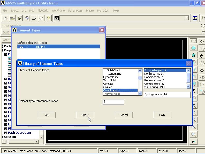
COMBIN14 is added to the Element Types window.

Click OK to close Library of Element Types window.

Then in Element Types window select COMBIN14 and click on Options button.

COMBIN14 element type options window appears. From DOF selection for 2D + 3D list select 2-D longitudinal option and click OK.

Next we must define the mass element. In Element Types window click on Add button. Library of Element Types window appears. From left column select Structural Mass and from right column select 3D mass 21 and click OK.

MASS21 is added to the Element Types window.

Select MASS21 from list and click on Options button.

MASS21 element type options window appears. From Rotary inertia options list select 2-D w rot inert option and click OK. Then close Element Types window.

2). To define the Element Properties, from Main Menu click Preprocessor - Real Constants - Add/Edit/Delete. Real Constants window appears. Click on Add button.

Then from list select COMBIN14 and click OK.

Real Constant Set Number 1, for COMBIN14 window appears. In Spring constant box enter 2400 then click OK.

Set 1 is added to the Real Constants window.

Again in Real Constants window click on Add button. From list select BEAM3 and click OK.

Real Constants for BEAM3 window appears. In Cross sectional area, Area moment of inertia, and Total beam height boxes enter 1 and click OK.

Set 2 is added to Real Constants window.

In Real Constants window click on Add button. Then from list select MASS21 and click OK.

Real Constant Set Number 3, for MASS21 window appears. In 2-D mass box enter 100 and click OK.

Set 3 is added to the Real Constants window.

To define the beam and spring element properties of the right side section of the system, in Real Constants window click on Add button and from list select BEAM3 and click OK.

Real Constants for BEAM3 window appears. In Cross sectional area, Area moment of inertia, and Total beam height boxes enter 1 and click OK.

Set 4 is added to the Real Constants window.

Then in Real Constants window click on Add button. From list select COMBIN14 and click OK.

Real Constant Set Number 5, for COMBIN14 window appears. In Spring constant box enter 2600 and click OK.

Set 5 is added to the Real Constants window. Close this window.

3). To define Material Properties, from Main Menu click Preprocessor - Material Props - Material Models - Define Material Model Behavior window appears. Select Structural - Linear - Elastic - Isotropic. Enter EX = 4e9 and click OK.

Close Define Material Model Behavior window.

4). To create the Model, the direct modeling method is used. In this method nodes and elements are directly created and there is no need to do meshing.
From Main Menu click Preprocessor - Modeling - Create - Nodes - In Active CS. Create Nodes in Active Coordinate System window appears.

Create the following nodes:

The nodes are created.

In next stage the elements through these nodes are created. First from Main Menu click Preprocessor - Meshing - Mesh Attributes - Default Attribs. Meshing Attributes window appears. Use the following table to define the Elements.

From first list select COMBIN14 and from second and third list select 1 and click OK.

To create the left spring element, from Main Menu click Preprocessor - Modeling - Create - Elements - Auto Numbered - Thru Nodes. Elements from Nodes window appears. Pick nodes 1 and 2 and click OK.


From Main Menu click Preprocessor - Meshing - Mesh Attributes - Default Attribs. Meshing Attributes window appears. From first list select BEAM3 and from second select 1 and from third list select 2 and click OK.

To create the left beam element, from Main Menu click Preprocessor - Modeling - Create - Elements - Auto Numbered - Thru Nodes. Elements from Nodes window appears. Pick nodes 2 and 3 and click OK.


From Main Menu click Preprocessor - Meshing - Mesh Attributes - Default Attribs. Meshing Attributes window appears. From first list select MASS21 and from second select 1 and from third list select 3 and click OK.

To create the Mass Element, from Main Menu click Preprocessor - Modeling - Create - Elements - Auto Numbered - Thru Nodes. Elements from Nodes window appears. Pick node number 3 twice and click OK.

From Main Menu click Preprocessor - Meshing - Mesh Attributes - Default Attribs. Meshing Attributes window appears. From first list select BEAM3 and from second select 1 and from third list select 4 and click OK.
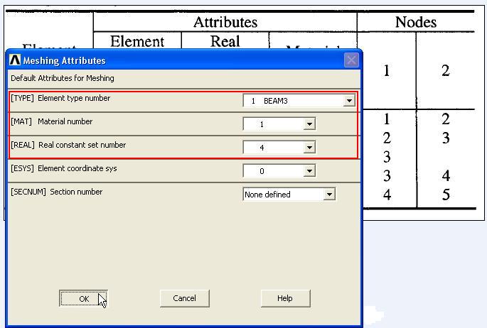
To create the right beam element, from Main Menu click Preprocessor - Modeling - Create - Elements - Auto Numbered - Thru Nodes. Elements from Nodes window appears. Pick nodes number 3 and 4 and click OK.


From Main Menu click Preprocessor - Meshing - Mesh Attributes - Default Attribs. Meshing Attributes window appears. From first list select COMBIN14 and from second select 1 and from third list select 5 and click OK.

To create the right spring element, from Main Menu click Preprocessor - Modeling - Create - Elements - Auto Numbered - Thru Nodes. Elements from Nodes window appears. Pick nodes number 4 and 5 and click OK.


Next from Menu click List - Elements - Nodes + Attributes.

A table of element attributes appears.

5). To define Analysis Type, from Main Menu click Solution - Analysis Type - New Analysis. New Analysis window appears. Select Modal option and click OK.

From Main Menu click Solution - Analysis Type - Analysis Options. Modal Analysis window appears. For Mode extraction method select Reduced option. In No. of modes to extract box enter 2 and click OK.
NOTE: This method employs the use of Master Degrees of Freedom. These are degrees of freedom that govern the dynamic characteristics of a structure. This is the fastest method as it reduces the system matrices to only consider the Master Degrees of Freedom. The Subspace Method extracts modes for all DOF's. It is therefore more exact but, it also takes longer to compute (especially when the complex geometries).

Reduced Modal Analysis window appears. In Frequency range boxes enter 0 and 10 respectively. Click OK.

In next stage we need to define the Master Degrees of Freedom (MDOF's) of this system. From Main Menu click Solution - Master DOFs - User Selected - Define. Define Master DOFs window appears. Pick node number 3 and click OK.

Define Master DOFs window appears. From first list select UY and from second list select ROTZ and click OK.

From Main Menu click Solution - Load Step Opts - Output Ctrls - Solu Printout. Solution Printout Controls window appears. From first list select Nodal DOF solu option. Then select Every substep option. Click OK.

From Main Menu click Solution - Load Step Opts - ExpansionPass - Single Expand - Expand Modes. Expand Modes window appears. In No. of modes to expand box enter 2 and click OK.

6). To define Boundary Conditions, from Main Menu click Preprocessor - Loads - Define Loads - Apply - Structural - Displacement - On Nodes. Apply U, ROT on Nodes window appears. Pick nodes number 1 and 5 and click OK.

Apply U, ROT on Nodes window appears. From list select UX and UY and click OK.

From Main Menu click Preprocessor - Loads - Define Loads - Apply - Structural - Displacement - On Nodes. Apply U, ROT on Nodes window appears. Pick node number 3 and click OK.

Apply U, ROT on Nodes window appears. From list select UX and click OK.

===========================================================
Solution Stage:
From Main Menu click Solution - Solve - Current LS. Click OK to start solution. Close the window.

===========================================================
Post Processing Stage:
To view the first mode shape, from Main Menu click General Postproc - Read Results - First Set.

Then from Main Menu click General Postproc - Plot Results - Deformed Shape. Plot Deformed Shape window appears. Select Def + undeformed option and click OK.
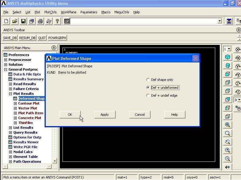
The frequency of the first mode is 1.098 Hz.

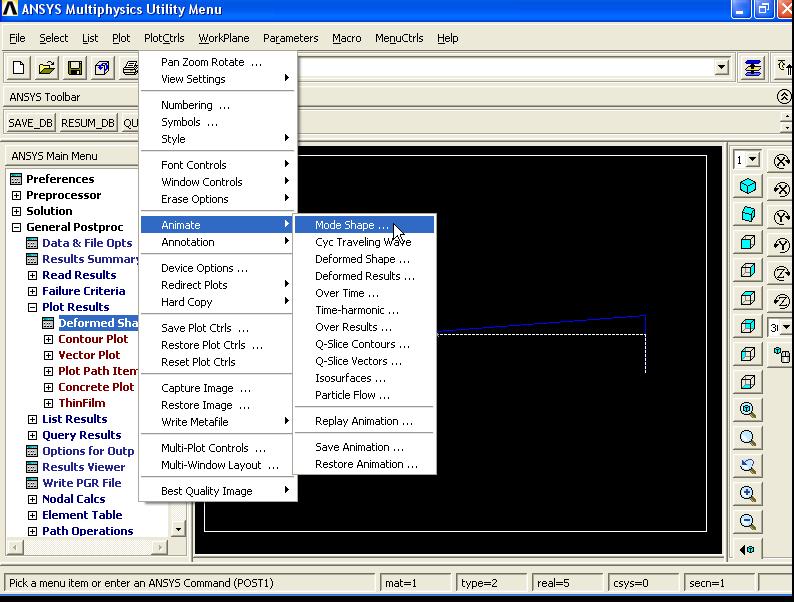
To animate the deformation, from Menu click PlotCtrls - Animate - Mode Shape.

Animate Mode Shape window appears. From left column select DOF Solution and from right column select Def + undeformed option and click OK.


Mode Shape 2: From Main Menu click General Postproc - Read Results - Next Set.

Then from Main Menu click General Postproc - Plot Results - Deformed Shape. Plot Deformed Shape window appears. Select Def + undeformed option and click OK.

The frequency of the second mode is 1.441 Hz.

To animate the deformation, from Menu click PlotCtrls - Animate - Mode Shape.
Animate Mode Shape window appears. From left column select DOF Solution and from right column select Def + undeformed option and click OK.


==========================================================
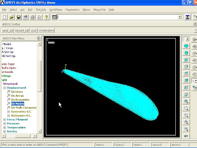
The coordinates of the wing is in Meter unit. The wing is fixed at one end. The aim is to find the first 5 mode natural frequencies of the wing and their corresponding deformed shapes. The wing is made of steel and E = 210GPa. Density = 7850Kg/m^3.

1). To define Element Type, from Main Menu click Preprocessor - Element Type - Add/Edit/Delete. Element Types window appears. Click on Add button. Library of Element Types window appears. From left column select Solid and from right column select 8node 82 and click Apply.

PLANE82 is added to the Element Types window.

Again from Library of Element Types window, from left column select Solid and from right column select Brick 8node 45 and click OK.

SOLID45 and PLANE82 are added to the Element Types list. Close this window.

2). To define Material Properties, from Main Menu click Preprocessor - Material Props - Material Models. Define Material Model Behavior window appears. From list select Structural - Linear - Elastic - Isotropic. Enter EX = 210e9 and PRXY = 0.3 and click OK.

To define Density, in Define Material Model Behavior window click Structural - Density. Enter DENS = 7850. Click OK.

Close Define Material Model Behavior window.

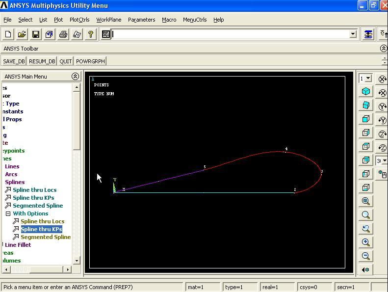
3). To create the Geometry, from Main Menu click Preprocessor - Modeling - Create - Keypoints - In Active CS. Create the following points: 1.(0,0,0) - 2.(2,0,0) - 3.(2.3,0.2,0) - 4.(1.9,0.45,0) - 5.(1,0.25,0) and click OK.
 To connect the points, from Main Menu click Preprocessor - Modeling - Create - Lines - Lines - In Active Coord. Lines in Active Coord window appears. Connect point 1 to point 2, and point1 to 5 as shown in figure. Then click OK.

To create the connecting splines of the other point, from Main Menu click Preprocessor - Modeling - Create - Lines - Splines - With Options - Spline thru KPs. B-Spline window appears. Then pick points number 2,3,4,5 as shown in figure and click OK.

B-Spline window appears. Enter XV1 = -1, XV6 = -1, YV6 = -0.25 and click OK.


To create the areas passing through the lines, from Main Menu click Preprocessor - Modeling - Create - Areas - Arbitrary - By Lines. Create Area by Lines window appears. Pick all the lines and click OK.


4). To Mesh the model, from Main Menu click Preprocessor - Meshing - Size Cntrls - ManualSize - Global - Size. Global Element Sizes window appears. In Element edge length box enter 0.05m and click OK.

Next from Main Menu click Preprocessor - Meshing - Mesh - Areas - Free. Mesh Areas window appears. Pick the area and click OK.


In next stage the model is extruded perpendicular to the area and a 3D model with its corresponding mesh is created. From Main Menu click Preprocessor - Modeling - Operate - Extrude - Elem Ext Opts. Element Extrusion Options window appears. From Element type number list select SOLID45 and in No. Elem divs box enter 10 and click OK.

From Main Menu click Preprocessor - Modeling - Operate - Extrude - Areas - Along Normal. Extrude Area by Norm window appears. Pick the area and click OK.

Extrude Area along Normal window appears. In Length of extrusion box enter 10 and click OK.


5). To apply Boundary Conditions, first we must deselect 2D elements (PLANE82). To do this, from Menu click Select Entities... Select Entities window appears. From first list select Elements and from second list select By Attributes. Then from next list select Elem type num option. In Min,Max,Inc box enter 1 then select Unselect option and click OK.

Then from Menu click Select - Entities. Select Entities window appears. From first list select Nodes and from second list select By Location then select Z coordinates option. In Min, Max box enter 0 and next select From Full option and click OK.

Now from Menu click Plot - Nodes. All the selected nodes are displayed.

From Main Menu click Preprocessor - Loads - Define Loads - Apply - Structural - Displacement - On Nodes. Apply U, ROT on Nodes window appears. Click on Pick All button.

Apply U, ROT on Nodes window appears. From list select All DOF and click OK.

From Menu click Select - Everything. Then from Menu click Plot - Elements.

6). To define Analysis Type, from Main Menu click Solution - Analysis Type - New Analysis. New Analysis window appears. From options select Modal and click OK.

Then from Main Menu click Solution - Analysis Type - Analysis Options. Modal Analysis window appears. Select Block Lanczos option. In No. of modes to extract box enter 5 and click OK.

Block Lanczos Method window appears. Enter Start Frequency = 0 and End Frequency = 2000 and click OK.

===========================================================
Solution Stage:
From Main Menu click Solution - Solve - Current LS. Click OK to start solution. Close the window.

===========================================================
Post Processing Stage:
To view first mode shape, from Main Menu click General Postproc - Read Results - First Set.

Then from Main Menu click General Postproc - Plot Results - Deformed Shape. Plot Deformed Shape window appears. Select Def + undeformed option and click OK.

The frequency of the first mode is 3.088 Hz.

Then from Main Menu click General Postproc - Plot Results - Contour Plot - Nodal Solu. Contour Nodal Solution Data window appears. From DOF Solution select Displacement vector sum option and click OK.


To animate the deformation, from Menu click PlotCtrls - Animate - Mode Shape...

Animate Mode Shape window appears. From left column select DOF Solution and from right column select Def + undef edge option and click OK.


Mode Shape 2: from Main Menu click General Postproc - Read Results - Next Set.

Then from Main Menu click General Postproc - Plot Results - Deformed Shape. Plot Deformed Shape window appears. Select Def + undef edge option and click OK.


To animate the deformation, from Menu click PlotCtrls - Animate - Mode Shape...

Animate Mode Shape window appears. From left column select DOF Solution and from right column select Def + undef edge option and click OK.


Mode Shape 3: from Main Menu click General Postproc - Read Results - Next Set.

Then from Main Menu click General Postproc - Plot Results - Deformed Shape. Plot Deformed Shape window appears. Select Def + undef edge option and click OK.


To animate the deformation, from Menu click PlotCtrls - Animate - Mode Shape...

Animate Mode Shape window appears. From left column select DOF Solution and from right column select Def + undef edge option and click OK.


Mode Shape 4: from Main Menu click General Postproc - Read Results - Next Set.

Then from Main Menu click General Postproc - Plot Results - Deformed Shape. Plot Deformed Shape window appears. Select Def + undef edge option and click OK.


To animate the deformation, from Menu click PlotCtrls - Animate - Mode Shape...

Animate Mode Shape window appears. From left column select DOF Solution and from right column select Def + undef edge option and click OK.


2). To define Material Properties, from Main Menu click Preprocessor - Material Props - Material Models. The window Define Material Model Behavior opens. Click on Structural - Linear - Elastic - Isotropic. Enter EX = 206e9 and PRXY = 0.3. Click OK.

To define density, click on Density term. Input the value of 7800 to DENS and click OK.

Two items as Density and Linear Isotropic are added to the list. Close this window.

3). To create the Geometry, from Main Menu click Preprocessor - Modeling - Create - Keypoints - In Active CS. The window Create Keypoints in Active Coordinate System opens. Input A 0,0 to X,Y,Z Location in active CS box, and then click Apply button. Do not click OK button at this stage. Create the following keypoints.


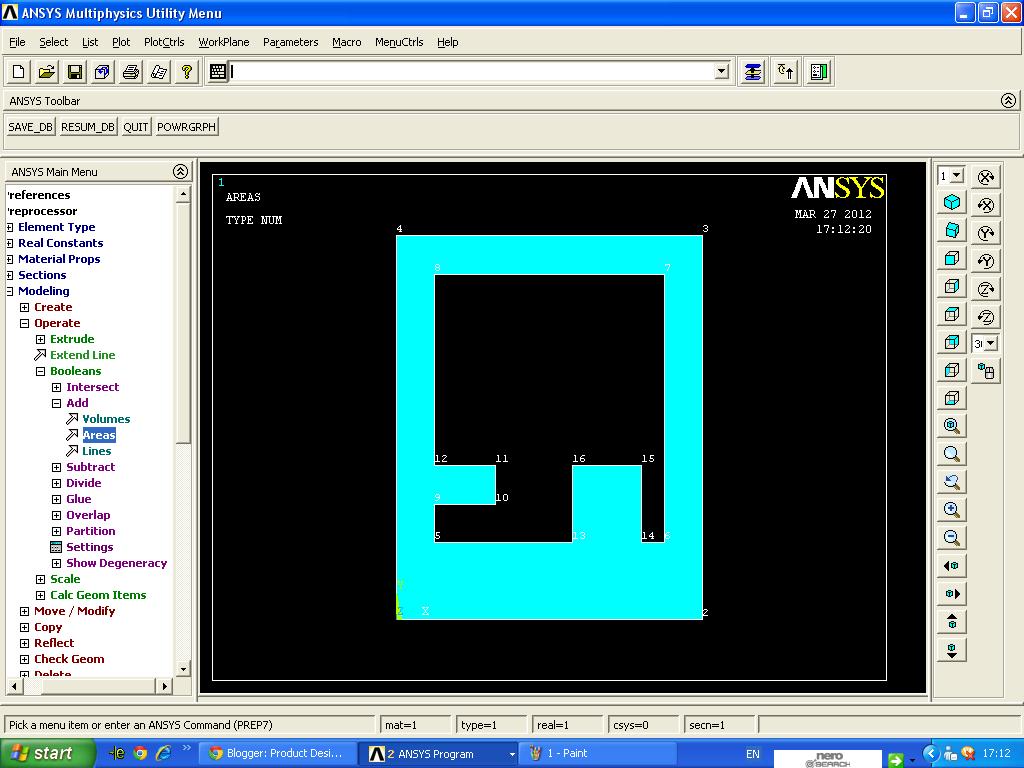
Areas are created from keypoints by clicking on Main Menu - Preprocessor - Modeling - Create - Areas - Arbitrary - Through KPs. The window Create Area thru KPs opens. Pick the keypoints, 1, 2, 3, and 4 in order and click Apply button. Then pick keypoints 5, 6, 7, and 8 and click OK button.


To remove the area, from Main Menu click Preprocessor - Modeling - Operate - Booleans - Subtract - Areas. Click the area of KP No. 1-4 and OK button. Then click the area of KP No. 5-8 and OK button.


The drawing of the table is as following figure.

Again from Main Menu click Preprocessor - Modeling - Create - Areas - Arbitrary - Through KPs. Pick keypoints 9, 10, 11, and 12 in order and click Apply button. Then pick keypoints 13, 14, 15, and 16 and click OK button.


From Main Menu click Preprocessor - Modeling - Operate - Booleans - Add - Areas. The window Add Areas opens. Pick three areas on graphic window and click OK. Then three areas are added.


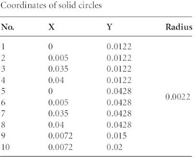
From Main Menu click Preprocessor - Modeling - Create - Areas - Circle - Solid Circle. The window Solid Circle Area opens. Input the values of 0, 12.2e-3, 2.2e-3 to X, Y and Radius boxes.


Then continue to input the coordinates of the solid circle as shown in table below. The radius of all solid circles is 0.0022. When all values are inputted, the drawing of the table appears as image below.

From Main Menu click Preprocessor - Modeling - Operate - Booleans - Subtract - Areas. Subtract all circular areas from the rectangular area. First select the rectangular area and click OK.

Then pick the circles and click OK.


4). To Mesh the area, from Main Menu click Preprocessor - Meshing - Mesh Tool. The window Mesh Tool opens. Click Lines Set and the window Element Size on Picked Lines opens.

Click Pick All button.

The window Element Sizes on Picked Lines opens. Input 0.001 to SIZE box and click OK.

Click Mesh of the window Mesh Tool and then the window Mesh Areas opens.

Pick the area of the table on graphics window and click OK.


Next, by performing the following steps, the thickness of 5 mm and the mesh size are determined for the drawing of the table.
From Main Menu click Preprocessor - Modeling - Operate - Extrude - Elem Ext Opts. The window Element Extrusion Options opens. Select SOLID45 from Element type number list and enter 5 in No. Elem divs and click OK.

From Main Menu click Preprocessor - Modeling - Operate - Extrude - Areas - By XYZ Offset. The window Extrude Area by Offset opens. Pick the area of the table on ANSYS Graphics window and click OK.

Then the window Extrude Areas by XYZ Offset opens. Input 0, 0, 0.005 to DX, DY, DZ boxes and click OK.


5). The table is fixed at both the bottom and the region A of the table. To apply Boundary Conditions, from Main Menu click Solution - Define Loads - Apply - Structural - Displacement - On Areas. The window Apply U, ROT on Areas opens. Pick the side wall for a piezoelectric actuator and the bottom of the table. Then click OK.

The window Apply U, ROT on Areas opens. Select All DOF in the box of Lab2 and then click OK.

6). To define the Type of Analysis, from Main Menu click Solution - Analysis Type - New Analysis. The window New Analysis opens. Check Modal and then click OK.

7). In order to define the number of modes to extract, from Main Menu click Solution - Analysis Type - Analysis Options. The window Modal Analysis opens. Check PCG Lanczos of MODOPT and input 3 in the box of No. of modes to extract and click OK.

The window PCG Lanczos Modal Analysis opens. Input 5000 in the box of End frequency and click OK.

8). Solution Stage: From Main Menu click Solution - Solve - Current LS. The window Solve Current Load Step opens. Click OK button and calculation starts. When the window Note appears, the calculation is finished.

Close the Note window.

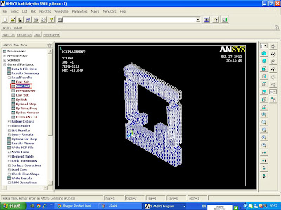
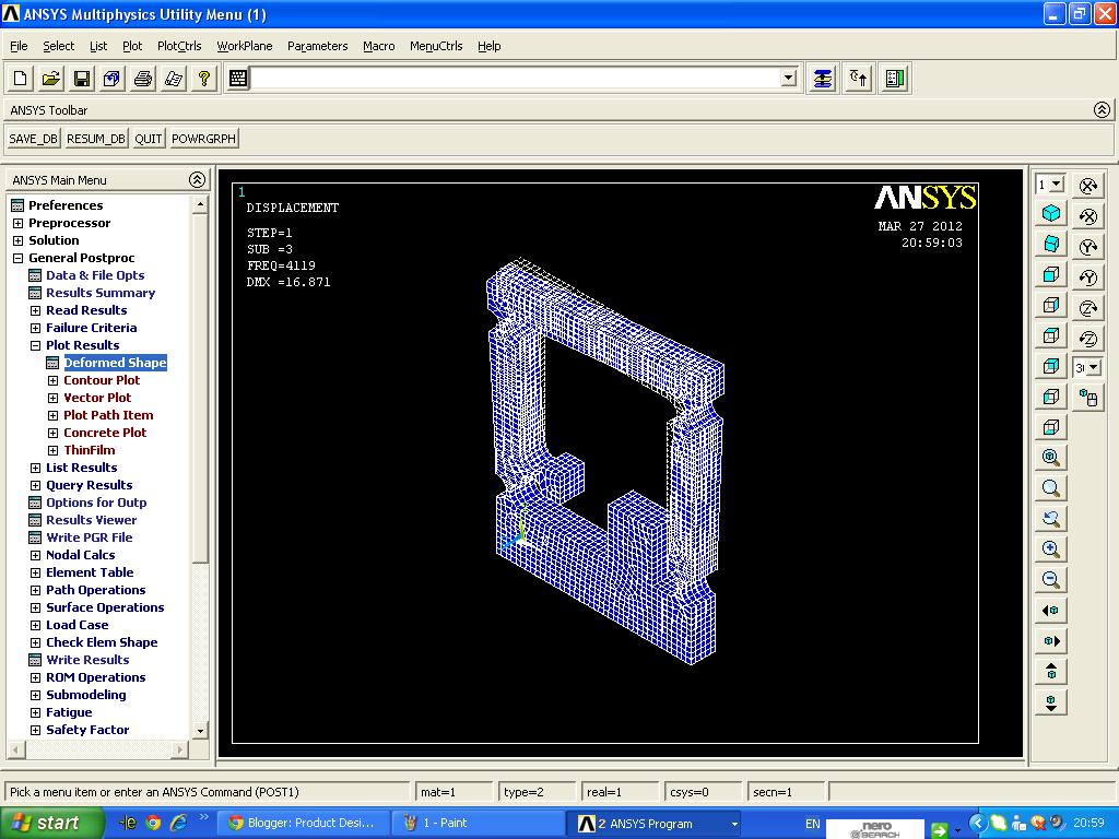
9). Post Processing stage: To read the calculated results of the first mode of vibration, from Main Menu click General Postproc - Read Results - First Set.

Then from Main Menu click General Postproc - Plot Results - Deformed Shape. The window Plot Deformed Shape opens. Select Def + Undeformed and click OK.

The first mode shape frequency is 1529 Hz.

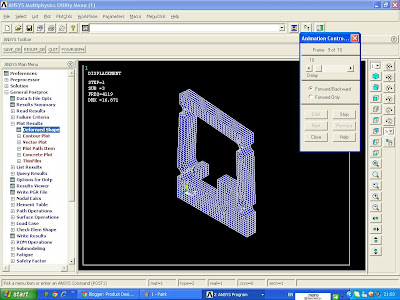
Second mode shape: From Main Menu click General Postproc - Read Results - Next Set.

Then from Main Menu click General Postproc - Plot Results - Deformed Shape.The window Plot Deformed Shape opens. Select Def + Undeformed and click OK.


Third mode shape: From Main Menu click General Postproc - Read Results - Next Set.
Then from Main Menu click General Postproc - Plot Results - Deformed Shape.The window Plot Deformed Shape opens. Select Def + Undeformed and click OK.


To animate the vibration mode shape, from Menu click PlotCtrls - Animate - Mode Shape.

The window Animate Mode Shape opens. Input 0.1 to Time delay box and click OK.


PLANE82 is added to the Element Types window.

Again from Library of Element Types window, from left column select Solid and from right column select Brick 8node 45 and click OK.

SOLID45 and PLANE82 are added to the Element Types list. Close this window.

2). To define Material Properties, from Main Menu click Preprocessor - Material Props - Material Models. Define Material Model Behavior window appears. From list select Structural - Linear - Elastic - Isotropic. Enter EX = 210e9 and PRXY = 0.3 and click OK.

To define Density, in Define Material Model Behavior window click Structural - Density. Enter DENS = 7850. Click OK.

Close Define Material Model Behavior window.

3). To create the Geometry, from Main Menu click Preprocessor - Modeling - Create - Keypoints - In Active CS. Create the following points: 1.(0,0,0) - 2.(2,0,0) - 3.(2.3,0.2,0) - 4.(1.9,0.45,0) - 5.(1,0.25,0) and click OK.


To create the connecting splines of the other point, from Main Menu click Preprocessor - Modeling - Create - Lines - Splines - With Options - Spline thru KPs. B-Spline window appears. Then pick points number 2,3,4,5 as shown in figure and click OK.

B-Spline window appears. Enter XV1 = -1, XV6 = -1, YV6 = -0.25 and click OK.

To create the areas passing through the lines, from Main Menu click Preprocessor - Modeling - Create - Areas - Arbitrary - By Lines. Create Area by Lines window appears. Pick all the lines and click OK.


4). To Mesh the model, from Main Menu click Preprocessor - Meshing - Size Cntrls - ManualSize - Global - Size. Global Element Sizes window appears. In Element edge length box enter 0.05m and click OK.

Next from Main Menu click Preprocessor - Meshing - Mesh - Areas - Free. Mesh Areas window appears. Pick the area and click OK.


In next stage the model is extruded perpendicular to the area and a 3D model with its corresponding mesh is created. From Main Menu click Preprocessor - Modeling - Operate - Extrude - Elem Ext Opts. Element Extrusion Options window appears. From Element type number list select SOLID45 and in No. Elem divs box enter 10 and click OK.

From Main Menu click Preprocessor - Modeling - Operate - Extrude - Areas - Along Normal. Extrude Area by Norm window appears. Pick the area and click OK.

Extrude Area along Normal window appears. In Length of extrusion box enter 10 and click OK.


5). To apply Boundary Conditions, first we must deselect 2D elements (PLANE82). To do this, from Menu click Select Entities... Select Entities window appears. From first list select Elements and from second list select By Attributes. Then from next list select Elem type num option. In Min,Max,Inc box enter 1 then select Unselect option and click OK.

Then from Menu click Select - Entities. Select Entities window appears. From first list select Nodes and from second list select By Location then select Z coordinates option. In Min, Max box enter 0 and next select From Full option and click OK.

Now from Menu click Plot - Nodes. All the selected nodes are displayed.

From Main Menu click Preprocessor - Loads - Define Loads - Apply - Structural - Displacement - On Nodes. Apply U, ROT on Nodes window appears. Click on Pick All button.

Apply U, ROT on Nodes window appears. From list select All DOF and click OK.


From Menu click Select - Everything. Then from Menu click Plot - Elements.

6). To define Analysis Type, from Main Menu click Solution - Analysis Type - New Analysis. New Analysis window appears. From options select Modal and click OK.

Then from Main Menu click Solution - Analysis Type - Analysis Options. Modal Analysis window appears. Select Block Lanczos option. In No. of modes to extract box enter 5 and click OK.

Block Lanczos Method window appears. Enter Start Frequency = 0 and End Frequency = 2000 and click OK.

===========================================================
Solution Stage:
From Main Menu click Solution - Solve - Current LS. Click OK to start solution. Close the window.

===========================================================
Post Processing Stage:
To view first mode shape, from Main Menu click General Postproc - Read Results - First Set.

Then from Main Menu click General Postproc - Plot Results - Deformed Shape. Plot Deformed Shape window appears. Select Def + undeformed option and click OK.

The frequency of the first mode is 3.088 Hz.

Then from Main Menu click General Postproc - Plot Results - Contour Plot - Nodal Solu. Contour Nodal Solution Data window appears. From DOF Solution select Displacement vector sum option and click OK.


To animate the deformation, from Menu click PlotCtrls - Animate - Mode Shape...

Animate Mode Shape window appears. From left column select DOF Solution and from right column select Def + undef edge option and click OK.


Mode Shape 2: from Main Menu click General Postproc - Read Results - Next Set.

Then from Main Menu click General Postproc - Plot Results - Deformed Shape. Plot Deformed Shape window appears. Select Def + undef edge option and click OK.


To animate the deformation, from Menu click PlotCtrls - Animate - Mode Shape...

Animate Mode Shape window appears. From left column select DOF Solution and from right column select Def + undef edge option and click OK.


Mode Shape 3: from Main Menu click General Postproc - Read Results - Next Set.

Then from Main Menu click General Postproc - Plot Results - Deformed Shape. Plot Deformed Shape window appears. Select Def + undef edge option and click OK.


To animate the deformation, from Menu click PlotCtrls - Animate - Mode Shape...

Animate Mode Shape window appears. From left column select DOF Solution and from right column select Def + undef edge option and click OK.


Mode Shape 4: from Main Menu click General Postproc - Read Results - Next Set.

Then from Main Menu click General Postproc - Plot Results - Deformed Shape. Plot Deformed Shape window appears. Select Def + undef edge option and click OK.


To animate the deformation, from Menu click PlotCtrls - Animate - Mode Shape...

Animate Mode Shape window appears. From left column select DOF Solution and from right column select Def + undef edge option and click OK.


===========================================================
===========================================================
Mode Analysis of a One-axis Precision Moving Table:
A one-axis table using elastic hinges has been often used in various precision equipment, and the position of a table is usually controlled at nanometre-order accuracy using a piezoelectric actuator or a voice coil motor. Therefore, it is necessary to confirm the resonant frequency in order to determine the controllable frequency region.
A one-axis table using elastic hinges has been often used in various precision equipment, and the position of a table is usually controlled at nanometre-order accuracy using a piezoelectric actuator or a voice coil motor. Therefore, it is necessary to confirm the resonant frequency in order to determine the controllable frequency region.
Obtain the resonant frequency of a one-axis moving table using elastic hinges when the bottom of the table is fixed and a piezoelectric actuator is selected as an actuator:
- Material: Steel, thickness of the table: 5mm
- Young's modulus, E = 206 GPa, Poisson's ratio v=0.3
- Density P = 7.8 x 10^3 Kg/m^3
- Boundary condition: All freedoms are constrained at the bottom of the table and the region A indicated in figure, where a piezoelectric actuator is glued

In this example, the solid element is selected to analyze the resonant frequency of the moving table.
1). To define Element Type, from Main Menu click Preprocessor - Element Type - Add/Edit/Delete. Element Types window appears.

Click on Add button. Then the window Library of Element Types opens. From left column select Solid and from right column select Quad 4node 42 and click Apply.

Then select Brick 8node 45 from right column and click OK.

PLANE42 and SOLID45 are added to the Element Types window. Close this window.

2). To define Material Properties, from Main Menu click Preprocessor - Material Props - Material Models. The window Define Material Model Behavior opens. Click on Structural - Linear - Elastic - Isotropic. Enter EX = 206e9 and PRXY = 0.3. Click OK.

To define density, click on Density term. Input the value of 7800 to DENS and click OK.

Two items as Density and Linear Isotropic are added to the list. Close this window.

3). To create the Geometry, from Main Menu click Preprocessor - Modeling - Create - Keypoints - In Active CS. The window Create Keypoints in Active Coordinate System opens. Input A 0,0 to X,Y,Z Location in active CS box, and then click Apply button. Do not click OK button at this stage. Create the following keypoints.


Areas are created from keypoints by clicking on Main Menu - Preprocessor - Modeling - Create - Areas - Arbitrary - Through KPs. The window Create Area thru KPs opens. Pick the keypoints, 1, 2, 3, and 4 in order and click Apply button. Then pick keypoints 5, 6, 7, and 8 and click OK button.


To remove the area, from Main Menu click Preprocessor - Modeling - Operate - Booleans - Subtract - Areas. Click the area of KP No. 1-4 and OK button. Then click the area of KP No. 5-8 and OK button.


The drawing of the table is as following figure.

Again from Main Menu click Preprocessor - Modeling - Create - Areas - Arbitrary - Through KPs. Pick keypoints 9, 10, 11, and 12 in order and click Apply button. Then pick keypoints 13, 14, 15, and 16 and click OK button.


From Main Menu click Preprocessor - Modeling - Operate - Booleans - Add - Areas. The window Add Areas opens. Pick three areas on graphic window and click OK. Then three areas are added.

From Main Menu click Preprocessor - Modeling - Create - Areas - Circle - Solid Circle. The window Solid Circle Area opens. Input the values of 0, 12.2e-3, 2.2e-3 to X, Y and Radius boxes.


Then continue to input the coordinates of the solid circle as shown in table below. The radius of all solid circles is 0.0022. When all values are inputted, the drawing of the table appears as image below.


From Main Menu click Preprocessor - Modeling - Operate - Booleans - Subtract - Areas. Subtract all circular areas from the rectangular area. First select the rectangular area and click OK.

Then pick the circles and click OK.


4). To Mesh the area, from Main Menu click Preprocessor - Meshing - Mesh Tool. The window Mesh Tool opens. Click Lines Set and the window Element Size on Picked Lines opens.

Click Pick All button.

The window Element Sizes on Picked Lines opens. Input 0.001 to SIZE box and click OK.

Click Mesh of the window Mesh Tool and then the window Mesh Areas opens.

Pick the area of the table on graphics window and click OK.


Next, by performing the following steps, the thickness of 5 mm and the mesh size are determined for the drawing of the table.
From Main Menu click Preprocessor - Modeling - Operate - Extrude - Elem Ext Opts. The window Element Extrusion Options opens. Select SOLID45 from Element type number list and enter 5 in No. Elem divs and click OK.

From Main Menu click Preprocessor - Modeling - Operate - Extrude - Areas - By XYZ Offset. The window Extrude Area by Offset opens. Pick the area of the table on ANSYS Graphics window and click OK.

Then the window Extrude Areas by XYZ Offset opens. Input 0, 0, 0.005 to DX, DY, DZ boxes and click OK.


5). The table is fixed at both the bottom and the region A of the table. To apply Boundary Conditions, from Main Menu click Solution - Define Loads - Apply - Structural - Displacement - On Areas. The window Apply U, ROT on Areas opens. Pick the side wall for a piezoelectric actuator and the bottom of the table. Then click OK.

The window Apply U, ROT on Areas opens. Select All DOF in the box of Lab2 and then click OK.

6). To define the Type of Analysis, from Main Menu click Solution - Analysis Type - New Analysis. The window New Analysis opens. Check Modal and then click OK.

7). In order to define the number of modes to extract, from Main Menu click Solution - Analysis Type - Analysis Options. The window Modal Analysis opens. Check PCG Lanczos of MODOPT and input 3 in the box of No. of modes to extract and click OK.

The window PCG Lanczos Modal Analysis opens. Input 5000 in the box of End frequency and click OK.

8). Solution Stage: From Main Menu click Solution - Solve - Current LS. The window Solve Current Load Step opens. Click OK button and calculation starts. When the window Note appears, the calculation is finished.

Close the Note window.

9). Post Processing stage: To read the calculated results of the first mode of vibration, from Main Menu click General Postproc - Read Results - First Set.

Then from Main Menu click General Postproc - Plot Results - Deformed Shape. The window Plot Deformed Shape opens. Select Def + Undeformed and click OK.

The first mode shape frequency is 1529 Hz.

Second mode shape: From Main Menu click General Postproc - Read Results - Next Set.

Then from Main Menu click General Postproc - Plot Results - Deformed Shape.The window Plot Deformed Shape opens. Select Def + Undeformed and click OK.


Third mode shape: From Main Menu click General Postproc - Read Results - Next Set.

Then from Main Menu click General Postproc - Plot Results - Deformed Shape.The window Plot Deformed Shape opens. Select Def + Undeformed and click OK.

To animate the vibration mode shape, from Menu click PlotCtrls - Animate - Mode Shape.

The window Animate Mode Shape opens. Input 0.1 to Time delay box and click OK.

