MATLAB Introductory Commands:
MATLAB as a Calculator
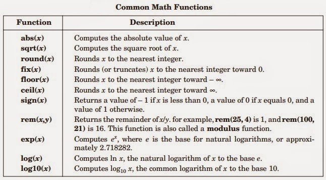
Mathematical Functions
Vector and Matrix Creation
Vector and Matrix Operations
Image Processing Toolbox
Converting Images
Spatial Image Filtering
Program Control
- What is MATLAB?
- The MATLAB Environment
- MATLAB Variables
- MATLAB as a Calculator
- Mathematical Functions
- Creating Vectors via Concatenation
- Creating Uniformly Spaced Vectors (Colon Operator)
- Complex Numbers
- Array Size and Length
- Vector Arithmetic
- Accessing Elements of a Vector
- Vector Transpose
- Line Plots
- Annotating Graphs
- Stem Plots
- For Loop
- Discrete Fourier Transform
- Creating Matrices
- Concatenating Arrays
- Array Creation Functions
- Accessing Elements of an Array
- Matrix Multiplication
- Logical Operators
- Calculating Eigenvalues and Eigenvectors
- Working with Classes
- Structure Arrays

Clear & clc commands:
Clear command clears the variables value. For example, in the example below, the value of the 4 is assigned to pi. By executing clear command the value of the pi is no longer 4 and now it is 3.1416.
clc command clear the screen and all the commands will disappear. By using Help command you can get information about any function.

By using Tab button you can complete the command you entered in MATLAB. For example, you enter ezp but you don't know the rest of the command so you can use Tab button to access a list commands that starts with ezp.
Help command:
who & whos commands:


In the example below, the linespace command will create 10 numbers between 0 and pi/2. The interval of the 10 numbers are equal.


Random Figure Generator:

The brackets in the example below, deletes the third elements of the array. Now the array r has 5 elements.

Matrix:


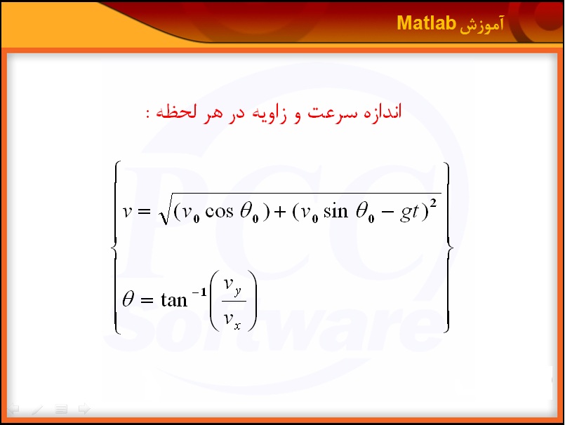
Vertical Motion under Gravity:


Linear equation examples:


Double Command: Double(x) returns the double-precision (Decimal) value for X.


To see other examples, click on Start button.

Select Demos option.


SUM command:

Disp command:

Format Command:


M-File:


To open the Editor:


For Loop:


Factorial and Limit calculation:


==========================================================
Introductory to structured programming (Projectile project):


% The proctile problem with zero air resistance
% in a gravitational field with constant g.
%
% An eight-step structure plan applied in MATLAB:
%
% 1. Definition of the input variables.
%
g = 9.81; % Gravity in m/s/s.
vo = input('What is the launch speed in m/s?')
tho = input('What is the launch angle in degrees?')
tho = pi*tho/180; % Conversion of degrees to radians.
%
% 2. Calculate the range and duration of the flight.
%
txmax = (2*vo/g) * sin(tho);
xmax = txmax * vo * cos(tho);
%
% 3. Calculate the sequence of time steps to compute trajectory.
%
dt = txmax/100;
t = 0:dt:txmax;
%
% 4. Compute the trajectory.
%
x = (vo * cos(tho)) .* t;
y = (vo * sin(tho)) .* t - (g/2) .* t.^2;
%
% 5. Compute the speed and angular direction of the projectile.
% Note that vx = dx/dt, vy = dy/dt.
%
vx = vo * cos(tho);
vy = vo * sin(tho) - g .* t;
v = sqrt(vx.*vx + vy.*vy);
th = (180/pi) .* atan2(vy,vx);
%
% 6. Compute the time, horizontal distance at maximum altitude.
%
tymax = (vo/g) * sin(tho);
xymax = xmax/2;
ymax = (vo/2) * tymax * sin(tho);
%
% 7. Display ouput.
%
disp(['Range in m = ',num2str(xmax),' Duration in s = ',...
num2str(txmax)])
disp(' ')
disp(['Maximum altitude in m = ',num2str(ymax), ...
' Arrival in s = ',num2str(tymax)])
plot(x,y,'k',xmax,y(size(t)),'o',xmax/2,ymax,'o')
title(['Projectile flight path, vo =',num2str(vo), ...
', th =', num2str(180*tho/pi)])
xlabel('x'), ylabel('y') % Plot of Figure 1.
axis('equal');
figure % Creates a new figure.
plot(v,th,'r')
title('Projectile speed vs. angle')
xlabel('V'), ylabel('\theta') % Plot of Figure 2.
%
% 8. Stop.
%


Structured Programming using functions (Projectile project):
function [xmax txmax] = projectile2(vo , tho)
% proctile problem with zero air resistance
% this is edited projectile problem
% that uses function to define the program
% in a gravitational field with constant g.
%
% An eight-step structure plan applied in MATLAB:
%
% 1. Definition of the input variables.
%
g = 9.81; % Gravity in m/s/s.
tho = pi*tho/180; % Conversion of degrees to radians.
%
% 2. Calculate the range and duration of the flight.
%
txmax = (2*vo/g) * sin(tho);
xmax = txmax * vo * cos(tho);
%
% 3. Calculate the sequence of time steps to compute trajectory.
%
dt = txmax/100;
t = 0:dt:txmax;
%
% 4. Compute the trajectory.
%
x = (vo * cos(tho)) .* t;
y = (vo * sin(tho)) .* t - (g/2) .* t.^2;
%
% 5. Compute the speed and angular direction of the projectile.
% Note that vx = dx/dt, vy = dy/dt.
%
vx = vo * cos(tho);
vy = vo * sin(tho) - g .* t;
v = sqrt(vx.*vx + vy.*vy);
th = (180/pi) .* atan2(vy,vx);
%
% 6. Compute the time, horizontal distance at maximum altitude.
%
tymax = (vo/g) * sin(tho);
ymax = (vo/2) * tymax * sin(tho);
%
% 7. Display ouput.
%
disp(['Range in m = ',num2str(xmax),' Duration in s = ',...
num2str(txmax)])
disp(' ')
disp(['Maximum altitude in m = ',num2str(ymax), ...
' Arrival in s = ',num2str(tymax)])
plot(x,y,'k',xmax,y(size(t)),'o',xmax/2,ymax,'o')
title(['Projectile flight path, vo =',num2str(vo), ...
', th =', num2str(180*tho/pi)])
xlabel('x'), ylabel('y') % Plot of Figure 1.
axis('equal');
figure % Creates a new figure.
plot(v,th,'r')
title('Projectile speed vs. angle')
xlabel('V'), ylabel('\theta') % Plot of Figure 2.
%
% 8. Stop.
%


Access to functions in MATLAB:


Functions:


Searching functions by using Help command:


Input & Output in MATLAB:


Saving Data in text string with ASCII format:


% Income tax the old-fashioned way 1
inc = [50000 100000 150000 300000 500000];
for ti = inc
if ti < 100000
tax = 0.1 * ti;
elseif ti < 200000
tax = 10000 + 0.2 * (ti - 100000);
else
tax = 30000 + 0.5 * (ti - 200000);
end;
disp( [ti tax] )
end;
inc = [50000 100000 150000 300000 500000];
for ti = inc
if ti < 100000
tax = 0.1 * ti;
elseif ti < 200000
tax = 10000 + 0.2 * (ti - 100000);
else
tax = 30000 + 0.5 * (ti - 200000);
end;
disp( [ti tax] )
end;
% Income tax the old-fashioned way 2
Income = input('What is your income?')
if Income<100000
tax = 0.1*Income;
elseif Income>100000&Income<200000
tax = 10000 + 0.2*(Income-100000);
elseif Income>200000
tax = 20000 + 0.5*(Income-200000);
end;
disp([Income tax]);
% Income tax the logical way
inc = [50000 100000 150000 300000 500000];
tax = 0.1 * inc .* (inc <= 100000);
tax = tax + (inc > 100000 & inc <= 200000) ...
.* (0.2 * (inc-100000) + 10000);
tax = tax + (inc > 200000) .* (0.5 * (inc-200000) + 30000);
disp( [inc' tax'] );
% This program computes n!
n = 10; % This line can be changed in order to change n!
fact = 1;
for k = 1:n
fact = k* fact;
end
disp([n fact]);
% This program computes the root of a real positive number
% and at the end shows the matlab's value for the root
format long
format compact
a = 2; % This line can be changed in order to change the results
x = a/2;
disp(['the approach to sqrt(a) for a= ' num2str(a)]);
for counter = 1:6
x = ( x + a/x)/2;
disp(x)
end
disp('Matlab''s value:')
disp(sqrt(a))
format
% This program computes the limit of the sequence
% a^k / k! for arbitrary k (say 20)
a =20; % This line can be changed to change a
k = 10; % Number of terms you can change this line
x = 1;
for n = 1:k
x = a*x/n;
disp([n x])
end
% This program use Selective structure method: Switch
d = floor(10*rand);
switch d
case {2, 4, 6, 8}
disp( 'Even' );
case {1, 3, 5, 7, 9}
disp( 'Odd' );
otherwise
disp( 'Zero' );
end
% This program creates a random integer number between 1 and 3 and displays the number in different cases
d = floor(3*rand) + 1
switch d
case 1
disp( 'That''s a 1!' );
case 2
disp( 'That''s a 2!' );
otherwise
disp( 'Must be 3!' );
end
=========================================================
MATLAB Logical Operations:


Calculation of current output of a Diode:


Plot sin(x)/x:


y = tan(x):


Examples:


==========================================================
MATLAB Matrix:


Application of (:) in matrix:


Copying and deleting rows and columns:


Primitive and special matrices:


Application of functions in matrices:


Matrices and For loop:


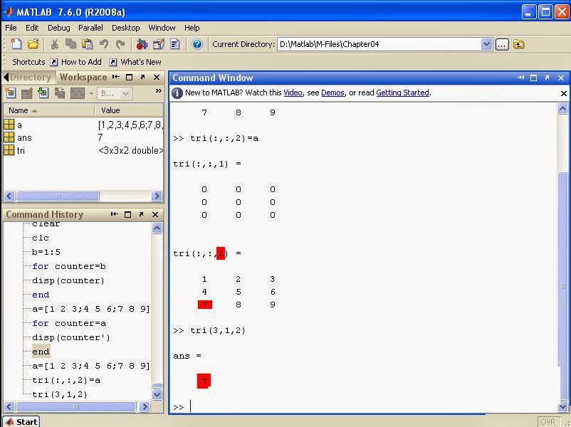
More dimensional matrices (3, 4, ...):


Product and power of matrices:


==========================================================
==========================================================Text Strings:


ASCII Codes:


Text Strings functions:


Two dimensional Text strings and execution:


===========================================================
===========================================================
MATLAB Graphic Foundations:


Labels:


Creating multi plots in one plot:


Line shape, Line color:


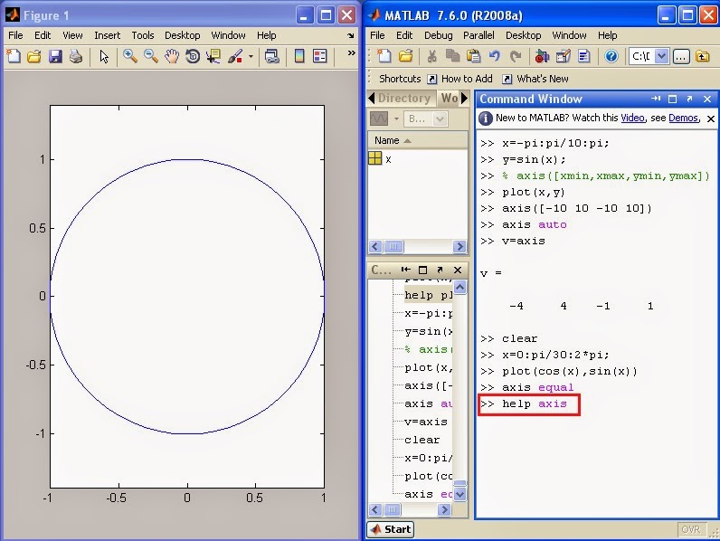
Plot Limits:


Creating multi plots in single window:


Defining a point by mouse:
Press Enter as well.


Number of points limited to 5 points.


Polar and Logarithmic Plots:


Plotting with rapid changes:


2 dimensional Graphic plots:


==========================================================
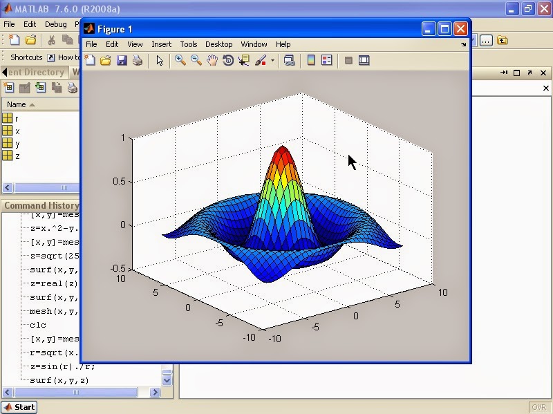
3 Dimension Graphics:


Creating Surfaces:


Changing surface domain by using NaN:


Contour Curves:


3D Dimensional Matrices:


3 Dimensional Graphic functions:


===========================================================
MATLAB Coding:
Function Categories:


Structure of function M-Files:


In one M-File you can define as many function as you can.

Workspaces:


Now we can use curve variable in two defined functions.
Various advanced data structure in MATLAB:


Cell Array data type:

=========================================================


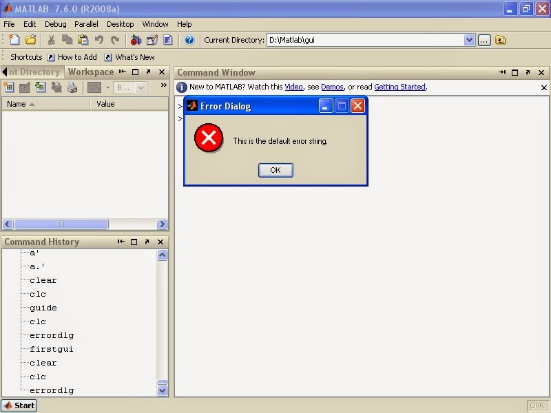
Click on OK.


Error Message:


Slider Control:


===========================================================
Matrix Main Functions:


Intersection of Rows and Columns:


Index into a matrix with a single index and MATLAB will handle it as if it was a vector using column-major order. Meaning that all the elements of one column are processed, in this case printed, before the elements of the next column. Column-major order is the default throughout MATLAB.


Meshgrid Function:

nargin & nargout Functions:
nargin is the number of input arguments and nargout is the number of output arguments that are in the user's calling statement.


Robustness:
A function declaration specifies:
- Name of the function
- Number of input arguments
- Number of output arguments
Function code and documentation specify:
- What the function does
- The type of the arguments
- What the arguments represent
Robustness:
- A function is robust if it handles erroneous input and output arguments
- Provides a meaningful error message


Persistent variable:
Variables:- Local
- Global
- Persistent
Persistent Variable:
- It's a local variable, but its value persists from one call of the function to the next
- Relatively rarely used
- None of the bad side effects of global variables
persistent X Y Z defines X, Y, and Z as variables that are local to the function in which they are declared; yet their values are retained in memory between calls to the function. Persistent variables are similar to global variables because the MATLAB software creates permanent storage for both. They differ from global variables in that persistent variables are known only to the function in which they are declared. This prevents persistent variables from being changed by other functions or from the MATLAB command line.
Whenever you clear or modify a function that is in memory, MATLAB also clears all persistent variables declared by that function. To keep a function in memory until MATLAB quits, use
mlock.
If the persistent variable does not exist the first time you issue the
persistent statement, it is initialized to the empty matrix.
It is an error to declare a variable persistent if a variable with the same name exists in the current workspace. MATLAB also errors if you declare any of a function's input or output arguments as persistent within that same function. For example, the following persistent declaration is invalid:
function myfun(argA, argB, argC)
persistent argB


The value of the persistent variable is initialized to an empty matrix by default. To retain the values in memory (buffer) between calls to the function, use the below code. This way the values will not be "lost" during repeated calls to the function.

Persistent variable example:


=====================================================
MATLAB Examples:


