Product Design Engineering: Harmonic Analysis of a Shell Bracket

The bracket is fixed to the wall through the top holes. The thickness of the plate is 0.1 inch. The bottom holes are under harmonic load (P) with range of +-1.5 pound and frequency range of 0 - 400 Hz. The aim is to produce the displacement graph of the middle point of bottom edge plate in terms of frequency of applied loads.

1). To define the Element Type, from Main Menu click Preprocessor - Element Type - Add/Edit/Delete. Element Types window appears. Click on Add button. Library of Element Types window appears. From left column select Shell and from right column select Elastic 4node 63 and click OK.

SHELL63 is added to the Element Types window. Close the window.

2). To define Element Properties, from Main Menu click Preprocessor - Real Constants - Add/Edit/Delete. Real Constants window appears. Click on Add button. Then click OK. Real Constant Set Number 1, for SHELL63 window appears. In Shell thickness at node I box enter 0.1inch and click OK.

Set 1 is added to the Real Constants list. Close this window.

3). To define Material Properties, from Main Menu click Preprocessor - Material Props - Material Models. Define Material Model Behavior window appears. Click Structural - Linear - Elastic - Isotropic. Enter EX = 3e7 and PRXY = 0.3 and click OK.

To define density, in Define Material Model Behavior window click Structural - Density. Enter DENS = 0.00073 and click OK.

Close Define Material Model Behavior window.

4). Before creating the Geometry we need to change the coordinate system. From Menu click WorkPlane - Offset WP by Increments. Offset WP window appears. In X,Y,Z Offsets box enter 0,3,-2 and click OK.

From Main Menu click Preprocessor - Modeling - Create - Areas - Rectangle - By Dimensions. Create Rectangle by Dimensions window appears. Enter X1 = -2 , X2 = 0, Y1 = 0, and Y2 = 2 and click OK.

From Main Menu click Preprocessor - Modeling - Create - Areas - Circle - By Dimensions. Circular Area by Dimensions window appears. Enter Outer radius = 1, Optional inner radius = 0, Starting angle (degrees) = 90, and Ending angle (degrees) = 180 and click OK.

Next we need to remove the circle from the rectangle. From Main Menu click Preprocessor - Modeling - Operate - Booleans - Subtract - Areas. Subtract Areas window appears. Pick the rectangle and click OK.

Then pick the circle and click OK.

Then we need to move the coordinate system to the centre of the top left hole. From Menu click WorkPlane - Offset WP by Increments. Offset WP window appears. In X,Y,Z Offsets box enter -1.5,1.5,0 and click OK.

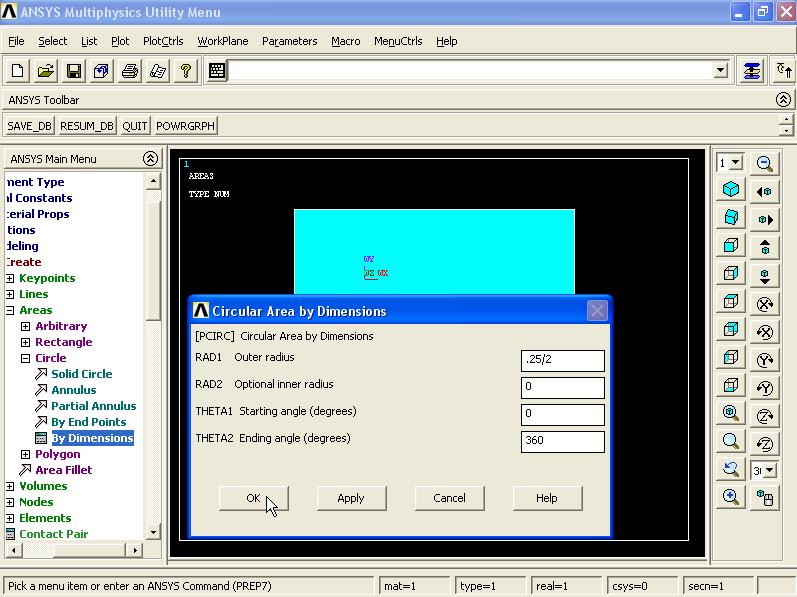
From Main Menu click Preprocessor - Modeling - Create - Areas - Circle - By Dimensions. Circular Area by Dimensions window appears. Enter Outer radius = 0.25/2, Optional inner radius = 0, Starting angle (degrees) = 0, and Ending angle (degrees) = 360 and click OK.

Next we need to remove the circle from the main area. From Main Menu click Preprocessor - Modeling - Operate - Booleans - Subtract - Areas. Subtract Areas window appears. Pick the main area and click OK.

Now pick the circle and click OK.

To create the rest of the model we need to change the coordinate system. From Menu click WorkPlane - Offset WP by Increments. Offset WP window appears. In X,Y,Z Offsets box enter -0.5,0.5,0 and click OK.

From Main Menu click Preprocessor - Modeling - Create - Areas - Rectangle - By Dimensions. Create Rectangle by Dimensions window appears. Enter X1 = 0, X2 = 1, Y1 = -2, and Y2 = -5 and click OK.

To create the curve end, from Main Menu click Preprocessor - Modeling - Create - Keypoints - In Active CS. Create the following points: 51.(0,0,0), 52.(-0.5,0,0) and click OK.

To create the end curve, from Main Menu click Preprocessor - Modeling - Operate - Extrude - Lines - About Axis. Sweep Lines about Axis window appears. Pick the line as shown in the figure and click OK.

Next define the sweep axis. In the box enter the point numbers as 51 and 52 and click OK.

Sweep Lines about Axis window appears. In Arc length in degrees box enter 45 and click OK.

In next stage we need to combine all the areas. From Main Menu click Preprocessor - Modeling - Operate - Booleans - Glue - Areas. Glue Areas window appears. Click on Pick All button.

Now we want to mirror the geometry and the mesh about Y-Z plane. From Main Menu click Preprocessor - Modeling - Reflect - Areas. Reflect Areas window appears. Pick the model and click OK.

Reflect Areas window appears. Select Y-Z plane option. Click OK.

Reflecting the geometry causes nodes, keypoints and rest of the model to overlap. In this situation we will encounter problems when applying boundary conditions and loading. To solve this problem, from Main Menu click Preprocessor - Numbering Ctrls - Merge Items. Merge Coincident of Equivalently Defined Items window appears. From the top list select All and click OK.

To create the rest of the model, from Menu click WorkPlane - Local Coordinate System - Create Local CS - At Specified Loc +.

Create CS at Location window appears. In the box enter 0,0,0 and click OK.

Create Local CS at Specified Location window appears. In Rotation about local X box enter -45 degree and click OK.

Now we want to mirror the whole geometry about X-Z plane of new local coordinate system. From Main Menu click Preprocessor - Modeling - Reflect - Areas. Reflect Areas window appears. Click Pick All button.

Reflect Areas window appears. Select X-Z Plane option. Click OK.

From Main Menu click Preprocessor - Numbering Ctrls - Merge Items. Merge Coincident of Equivalently Defined Items window appears. From the top list select All and click OK.

From Menu click Plot - Elements.

5). To Mesh the model, from Main Menu click Preprocessor - Meshing - Size Cntrls - ManualSize - Areas - All Areas. Element Sizes on All Selected Areas window appears. In Element edge length box enter 0.15inch and click OK.

Then from Main Menu click Preprocessor - Meshing - Mesh - Areas - Free. Mesh Areas window appears. Click on Pick All button.

===========================================================

Modal Analysis Stage:

6). From Main Menu click Solution - Analysis Type - New Analysis. New Analysis window appears. Then select Modal option and click OK.

From Main Menu click Solution - Analysis Type - Analysis Options. Modal Analysis window appears. Select Block Lanczos option. In No. of modes to extract box enter 5 and click OK.

Block Lanczos Method window appears. In Start frequency box enter 0 and in End frequency box enter 450 and click OK.

7). To apply Boundary Conditions, from Main Menu click Preprocessor - Loads - Define Loads - Apply - Structural - Displacement - On Nodes. Apply U, ROT on Nodes window appears. Pick all the top holes nodes as shown in figure. Click OK.

Apply U, ROT on Nodes window appears. From list select All DOF and click OK.

Now the modal analysis is ready to be solved. First from Menu click File - Save as Jobname.db.

Then from Main Menu click Solution - Solve - Current LS. Click OK to start solution. Then close the window.

After solution is finished from Main Menu click Finish.

===========================================================

Harmonic Analysis Stage:

From Main Menu click Solution - Analysis Type - New Analysis. New Analysis window appears. Select Harmonic option and click OK.

From Main Menu click Solution - Analysis Type - Analysis Options. Harmonic Analysis window appears. From first list select Full and from second list select Real + imaginary option and click OK.

Full Harmonic Analysis window appears. Do not change any options and click OK.

To apply Loads to the bottom holes, from Main Menu click Solution - Define Loads - Apply - Structural - Force/Moment - On Nodes. Apply F/M on Nodes window appears. Pick all the bottom holes edges nodes as shown in the figure. Click OK.

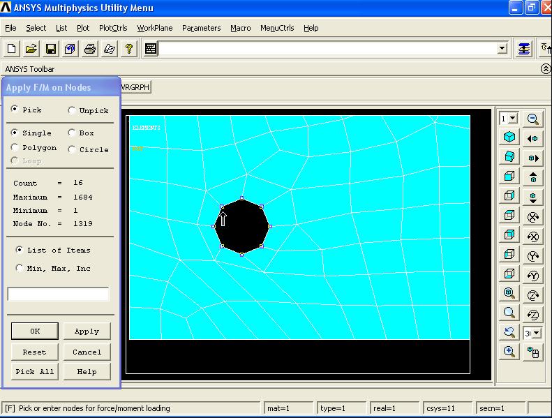
Apply F/M on Nodes window appears. From first list select FY and in Real part of force/mom box enter -3/8. 3N is the force and 8 is the number of nodes at each hole edge. Then click OK.

Then from Main Menu click Solution - Load Step Opts - Output Ctrls - Solu Printout. Solution Printout Controls window appears. From first list select All items option. Select Every substep option then click OK.

Then from Main Menu click Solution - Load Step Opts - Time/Frequenc - Freq and Substps. Harmonic Frequency and Substep Options window appears. In Harmonic freq range boxes enter 0 and 400 Hz. In Number of substeps box enter 100 and click OK.

Harmonic Solution Stage:

First from Menu click File - Save as Jobname.db.

Then from Main Menu click Solution - Solve - Current LS. Click OK to start solution. Then close the window.

After solution is finished from Main Menu click Finish.

Now the last step is to produce the displacement graph of the middle point of bottom edge plate in terms of frequency of applied loads.

From Main Menu click TimeHist Postproc. Time History Variables window appears. Click on Add Data button.

Add Time-History Variable window appears. Select Nodal Solution - DOF Solution - Y-Component of displacement. Click OK.

Node for Data window appears. Pick the middle bottom edge node as shown in the figure and click OK.

In Time History Variables window, click once on UY_2 (Y-Component of displacement) then click Graph Data button.

==========================================================

In a structural system, any sustained cyclic load will produce a sustained cyclic or harmonic response. Harmonic analysis results are used to determine the steady-state response of a linear structure to loads that vary sinusoidally (harmonically) with time, thus enabling you to verify whether or not your design will successfully overcome resonance, fatigue, and other harmful effects of forced vibrations.

In this analysis all loads as well as the structure’s response vary sinusoidally at the same frequency. A typical harmonic analysis will calculate the response of the structure to cyclic loads over a frequency range (a sine sweep) and obtain a graph of some response quantity (usually displacements) versus frequency. “Peak” responses are then identified from graphs of response vs. frequency and stresses are then reviewed at those peak frequencies.

In this example a steel wire with length of 700mm and diameter of 0.254mm is constrained at two end. This is done by applying a 84N horizontal force at right end node. A 1 N sinusoidal vertical force (F2) with 160mm distance from left end is applied. The frequency of the system is various and is between 0 and 2000 Hz. E = 190GPa. Density = 7920 Kg/m^3.

The aim is to find the displacement of the middle point of the wire in y direction in terms of frequency of the applied load and create the graph.

1). To define Element Type, from Main Menu click Preprocessor - Element Type - Add/Edit/Delete. Element Types window appears. Click on Add button. Library of Element Types window appears. From left column select Link and from right column select 2D Spar 1 and click OK.

LINK1 is added to the Element Types window. Close this window.

2). To define Element Properties, from Main Menu click Preprocessor - Real Constants - Add/Edit/Delete. Real Constants window appears. Click on Add button. LINK1 is added to the list then click OK.

Real Constant Set Number 1, for LINK1 window appears. In Cross-sectional area box enter 50671e-12 and click OK. Then close Real Constants window.

To define the density, in Define Material Model Behavior window, click Structural - Density. Enter DENS = 7920 and click OK.

Close Define Material Model Behavior window.

4). To create the Geometry, from Main Menu click Preprocessor - Modeling - Create - Keypoints - In Active CS. Create the following points: 1.(0,0,0) - 2.(0.7,0,0) and click OK.

Next two points must be connected together. From Main Menu click Preprocessor - Modeling - Create - Lines - Lines - Straight Line. Create Straight Line window appears. Pick the points and click OK. The points are connected.

5). To Mesh the model, from Main Menu click Preprocessor - Meshing - Mesh Tool. Mesh Tool window appears. Click on Lines Set button.

Element Size on Picked Lines window appears. Pick the line and click OK.

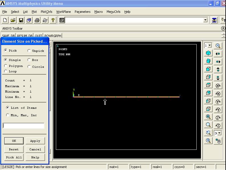
Element Sizes on Picked Lines window appears. In No. of element divisions box enter 35 and click OK.

In Mesh Tool window click on Mesh button.

Mesh Lines window appears. Pick the line and click OK.

To display the nodes, from Menu click Plot - Nodes.

Then from Menu click List - Nodes...

Sort NODE Listing window appears. Click OK.

The list of all nodes with their coordinates appears.

Node number 10 (X = 0.160, Y = 0, Z = 0) is the location where the harmonic load is applied.

Close the above window and from Menu click PlotCtrls - Numbering... Plot Numbering Controls window appears. Activate Node numbers option and click OK.

All the nodes are numbered.

Node number 10 is marked as shown in the figure.

NOTE: Before carrying out a Harmonic analysis, we must carry out first a Static analysis and then Modal analysis. After doing static and modal analysis, the Harmonic analysis is the final step.

6). To define Analysis Type, from Main Menu click Solution - Analysis Type - New Analysis. New Analysis window appears. Select Static option and click OK.

Apply U, ROT on Nodes window appears. From list select All DOF and click OK.

Then constrain rest of the nodes in y direction. From Main Menu click Preprocessor - Loads - Define Loads - Apply - Structural - Displacement - On Nodes. Apply U, ROT on Nodes window appears. Select the Box option from window and pick all the nodes except the left most node as shown in figure below. Click OK.

Apply U, ROT on Nodes window appears. From list select UY and click OK.

8). To define the Load from Main Menu click Preprocessor - Loads - Define Loads - Apply - Structural - Force/Moment - On Nodes. Apply F/M on Nodes window appears. Pick the last end node as shown in figure and click OK.

Apply F/M on Nodes window appears. From first list select FX and in Force/moment value box enter 84N and click OK.

9). From Main Menu click Solution - Analysis Type - Sol'n Controls. Solution Controls window appears. Enter Basic tab. Select Calculate prestress effects option. In Write Items to Results File section select All solution items. From Frequency: list select Write every substep option. Then click OK.

10). Then from Menu click File - Save as Jobname.db. By doing this the current analysis is active and considered.

===========================================================
Static Solution Stage:

11). From Main Menu click Solution - Solve - Current LS. Click OK to start solution. Then close the window.

Then from Main Menu click Finish option.

12). In next stage a Modal analysis will be carried out. To do this from Main Menu click Solution - Analysis Type - New Analysis. Select Modal and click OK.

Next from Main Menu click Solution - Analysis Type - Analysis Options. Modal Analysis window appears. Select Block Lanczos. In No. of modes to extract box enter 6. Then select Incl prestress effects? option and click OK.

Block Lanczos Method window appears. In Start Frequency box enter 0 and in End Frequency box enter 2000 and click OK.

13). Before modal analysis, we must delete all the nodes constraints (UY) except the end nodes. From Main Menu click Preprocessor - Loads - Define Loads - Delete - Structural - Displacement - On Nodes. Delete Node Constraints window appears. Select Box option from window and pick all the nodes except the both ends nodes.

Left end node is not selected.

And also right end node is not selected.

Delete Node Constraints window appears. From list select UY and click OK.

All the nodes constraints except both end nodes are deleted.

===========================================================
Modal Solution Stage:

Firs from Menu select Save as Jobname.db option.

Then from Main Menu click Solution - Solve - Current LS. Click OK to start solution and then close the window.

Then from Main Menu click Finish.

===========================================================
Harmonic Analysis Stage:

From Main Menu click Solution - Analysis Type - New Analysis. New Analysis window appears. Then select Harmonic option and click OK.

From Main Menu click Solution - Analysis Type - Analysis Options. Harmonic Analysis window appears. From first list select Mode Superpos'n and from second list select Amplitude + phase option and click OK.

Mode Sup Harmonic Analysis window appears. Then without changing anything click OK.

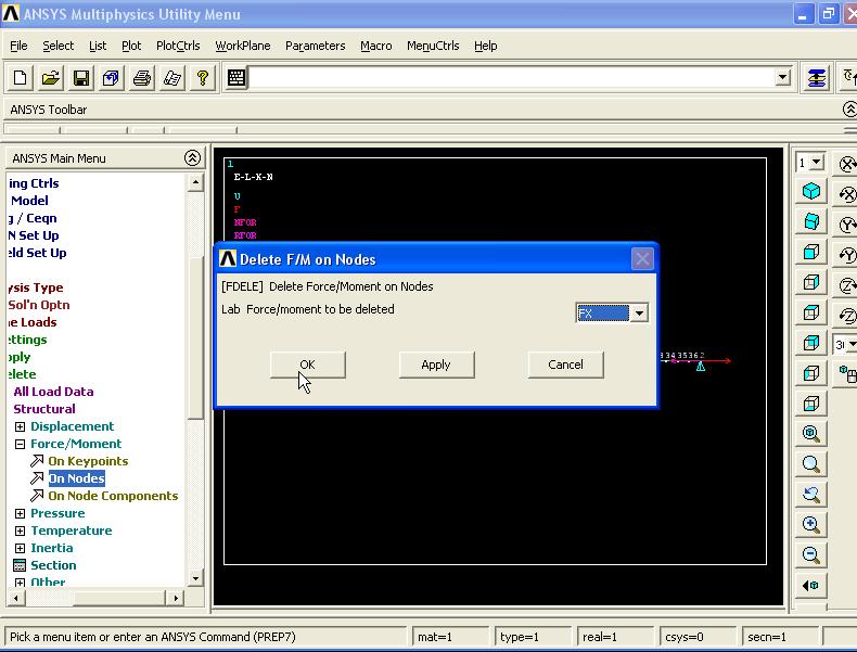
Then we must delete the horizontal load at right end node. From Main Menu click Preprocessor - Loads - Define Loads - Delete - Structural - Force/Moment - On Nodes. Delete F/M on Nodes window appears. Pick the right end node and click OK.

Delete F/M on Nodes window appears. From list select FX and click OK.

In next stage the vertical 1N force is applied. From Main Menu click Preprocessor - Loads - Define Loads - Apply - Structural - Force/Moment - On Nodes. Apply F/M on Nodes window appears. Pick node number 8 and click OK.

Apply F/M on Nodes window appears. From first list select FY and in Real part of force/mom box enter -1 and click OK.

In next stage from Main Menu click Solution - Load Step Opts - Time/Frequenc - Freq and Substps. Harmonic Frequency and Substep Options window appears. In Harmonic freq range enter 0 and 2000 and in Number of substeps box enter 250 and click OK.

Now the problem is ready to be solved in Harmonic mode. From Menu click File - Save as Jobname.db.

===========================================================
Harmonic Solution Stage:

Then from Main Menu click Solution - Solve - Current LS. Click OK to start solution. Then close the window.

Then from Main Menu click Finish.

To create the graph of the displacement of the middle point of the wire in y direction in terms of frequency of the applied load, from Main Menu click TimeHist Postpro. Time History Variables window appears. Click on Add Data button.