Transient Analysis:
Transient dynamic analysis (sometimes called time-history analysis) is a technique used to determine the dynamic response of a structure under the action of any general time-dependent loads. The ANSYS program uses the Newmark time integration method to solve these equations at discrete time points.
Transient structural that is also termed as time history load is the type of analysis in which time dependent loads are applied. Load varies from time to time. It is used for both linear as well as non linear analysis. Non linear transient involves large deformations, stresses, plasticity as well as cracks.
=========================================================
Exercise 1: Transient Analysis of a Shell Plate
The bracket is fixed to the wall through the top holes. The thickness of the plate is 0.1 inch.

According to the graph a 12N force in 0.005s is applied to the bottom left hole. The aim is to produce a graph of Displacement, Velocity, and Acceleration of left bottom corner of bracket in terms of Time.

1). To define the Element Type, from Main Menu click Preprocessor - Element Type - Add/Edit/Delete. Element Types window appears. Click on Add button. Library of Element Types window appears. From left column select Shell and from right column select Elastic 4node 63 and click OK.

SHELL63 is added to the Element Types window. Close the window.

2). To define Element Properties, from Main Menu click Preprocessor - Real Constants - Add/Edit/Delete. Real Constants window appears. Click on Add button. Then click OK. Real Constant Set Number 1, for SHELL63 window appears. In Shell thickness at node I box enter 0.1inch and click OK.

Set 1 is added to the Real Constants list. Close this window.

3). To define Material Properties, from Main Menu click Preprocessor - Material Props - Material Models. Define Material Model Behavior window appears. Click Structural - Linear - Elastic - Isotropic. Enter EX = 3e7 and PRXY = 0.3 and click OK.

To define density, in Define Material Model Behavior window click Structural - Density. Enter DENS = 0.00073 and click OK.

Close Define Material Model Behavior window.

4). Before creating the Geometry we need to change the coordinate system. From Menu click WorkPlane - Offset WP by Increments. Offset WP window appears. In X,Y,Z Offsets box enter 0,3,-2 and click OK.

From Main Menu click Preprocessor - Modeling - Create - Areas - Rectangle - By Dimensions. Create Rectangle by Dimensions window appears. Enter X1 = -2 , X2 = 0, Y1 = 0, and Y2 = 2 and click OK.


From Main Menu click Preprocessor - Modeling - Create - Areas - Circle - By Dimensions. Circular Area by Dimensions window appears. Enter Outer radius = 1, Optional inner radius = 0, Starting angle (degrees) = 90, and Ending angle (degrees) = 180 and click OK.


Next we need to remove the circle from the rectangle. From Main Menu click Preprocessor - Modeling - Operate - Booleans - Subtract - Areas. Subtract Areas window appears. Pick the rectangle and click OK.

Then pick the circle and click OK.


Then we need to move the coordinate system to the centre of the top left hole. From Menu click WorkPlane - Offset WP by Increments. Offset WP window appears. In X,Y,Z Offsets box enter -1.5,1.5,0 and click OK.


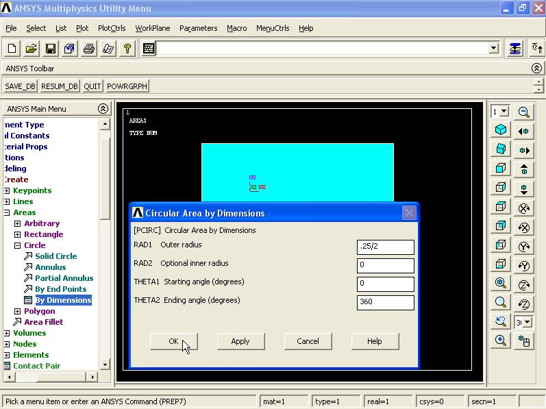
From Main Menu click Preprocessor - Modeling - Create - Areas - Circle - By Dimensions. Circular Area by Dimensions window appears. Enter Outer radius = 0.25/2, Optional inner radius = 0, Starting angle (degrees) = 0, and Ending angle (degrees) = 360 and click OK.

Next we need to remove the circle from the main area. From Main Menu click Preprocessor - Modeling - Operate - Booleans - Subtract - Areas. Subtract Areas window appears. Pick the main area and click OK.

Now pick the circle and click OK.


To create the rest of the model we need to change the coordinate system. From Menu click WorkPlane - Offset WP by Increments. Offset WP window appears. In X,Y,Z Offsets box enter -0.5,0.5,0 and click OK.


From Main Menu click Preprocessor - Modeling - Create - Areas - Rectangle - By Dimensions. Create Rectangle by Dimensions window appears. Enter X1 = 0, X2 = 1, Y1 = -2, and Y2 = -5 and click OK.


To create the curve end, from Main Menu click Preprocessor - Modeling - Create - Keypoints - In Active CS. Create the following points: 51.(0,0,0), 52.(-0.5,0,0) and click OK.


To create the end curve, from Main Menu click Preprocessor - Modeling - Operate - Extrude - Lines - About Axis. Sweep Lines about Axis window appears. Pick the line as shown in the figure and click OK.

Next define the sweep axis. In the box enter the point numbers as 51 and 52 and click OK.

Sweep Lines about Axis window appears. In Arc length in degrees box enter 45 and click OK.


In next stage we need to combine all the areas. From Main Menu click Preprocessor - Modeling - Operate - Booleans - Glue - Areas. Glue Areas window appears. Click on Pick All button.

Now we want to mirror the geometry and the mesh about Y-Z plane. From Main Menu click Preprocessor - Modeling - Reflect - Areas. Reflect Areas window appears. Pick the model and click OK.

Reflect Areas window appears. Select Y-Z plane option. Click OK.

Reflecting the geometry causes nodes, keypoints and rest of the model to overlap. In this situation we will encounter problems when applying boundary conditions and loading. To solve this problem, from Main Menu click Preprocessor - Numbering Ctrls - Merge Items. Merge Coincident of Equivalently Defined Items window appears. From the top list select All and click OK.

To create the rest of the model, from Menu click WorkPlane - Local Coordinate System - Create Local CS - At Specified Loc +.

Create CS at Location window appears. In the box enter 0,0,0 and click OK.

Create Local CS at Specified Location window appears. In Rotation about local X box enter -45 degree and click OK.


Now we want to mirror the whole geometry about X-Z plane of new local coordinate system. From Main Menu click Preprocessor - Modeling - Reflect - Areas. Reflect Areas window appears. Click Pick All button.

Reflect Areas window appears. Select X-Z Plane option. Click OK.


From Main Menu click Preprocessor - Numbering Ctrls - Merge Items. Merge Coincident of Equivalently Defined Items window appears. From the top list select All and click OK.

From Menu click Plot - Elements.

5). To Mesh the model, from Main Menu click Preprocessor - Meshing - Size Cntrls - ManualSize - Areas - All Areas. Element Sizes on All Selected Areas window appears. In Element edge length box enter 0.15inch and click OK.

Then from Main Menu click Preprocessor - Meshing - Mesh - Areas - Free. Mesh Areas window appears. Click on Pick All button.


===========================================================
Transient Analysis Stage:
6). From Main Menu click Solution - Analysis Type - New Analysis. New Analysis window appears. Select Transient option and click OK.

Transient Analysis window appears. Select Full option and click OK.

7). To apply Boundary Conditions, from Main Menu click Preprocessor - Loads - Define Loads - Apply - Structural - Displacement - On Nodes. Apply U, ROT on Nodes window appears. Pick all the top holes nodes as shown in figure. Click OK.


Apply U, ROT on Nodes window appears. From list select All DOF and click OK.

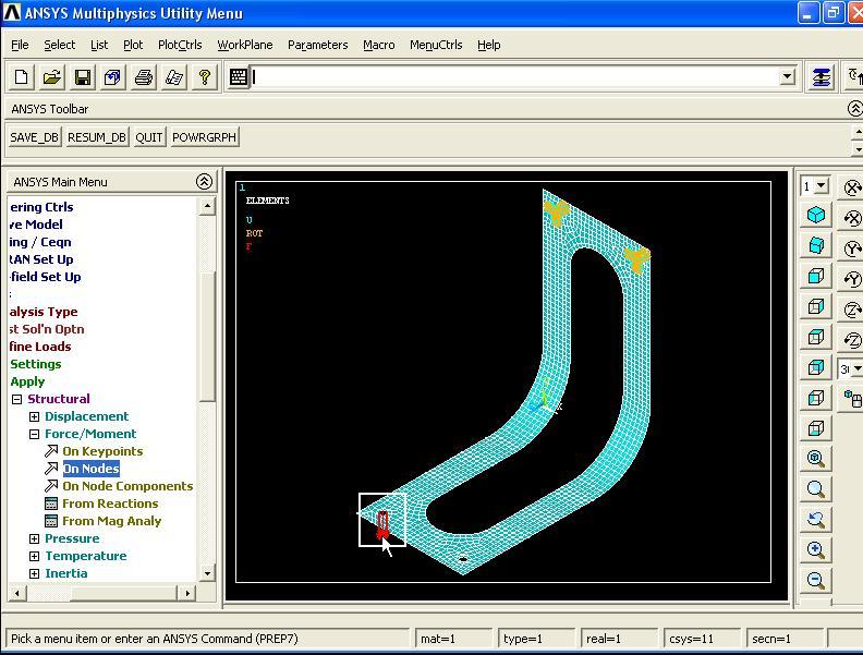
8). To apply the Force to the left bottom hole, from Main Menu click Preprocessor - Loads - Define Loads - Apply - Structural - Force/Moment - On Nodes. Apply F/M on Nodes window appears. From window select Circle option and pick all the hole edge nodes as shown in figure then click OK.

Apply F/M on Nodes window appears. From first list select FY and in Force/moment value box enter -12/8 (8 is the number of hole edge nodes) and click OK.

9). We want to solve the problem in three steps. This is done according to the F(t) graph. The 3 steps are based on time interval of: 1.(0 - 0.005s) - 2.(0.005 - 0.01) - 3.(0.01 - 0.1seconds). Each step is called Load step.

Step 1: From Main Menu click Solution - Analysis Type - Sol'n Controls - Solution Controls window appears. In Basic tab, enter 0.005s in Time at end of load step box. From Automatic time stepping list select On. Select Time increment option. In Time step size box enter 0.0001. Then select All solution items option. From Frequency: list select Write every substep.

Enter Transient tab in Solution Controls window. Select Ramped loading option and click OK.

Now the information related to the first step of loading must be saved. To do this, from Main Menu click Solution - Load Step Opts - Write LS File. Write Load Step File window appears. In Load step file number box enter 1 and click OK.

Step 2: For the second loading step in which the applied load reached 0, we must delete the applied load to the middle node. To do this from Main Menu click Solution - Define Loads - Delete - Structural - Force/Moment - On Nodes. Delete F/M on Nodes window appears. From window select Box option and pick all the hole edge nodes and click OK.

Delete F/M on Nodes window appears. From list select FY and click OK.

From Main Menu click Solution - Analysis Type - Sol'n Controls - Solution Controls window appears. In Basic tab, in Time at end of loadstep box enter 0.01s and click OK.

Now the information related to the second step of loading must be saved. To do this, from Main Menu click Solution - Load Step Opts - Write LS File. Write Load Step File window appears. In Load step file number box enter 2 and click OK.

Step 3: From Main Menu click Solution - Analysis Type - Sol'n Controls - Solution Controls window appears. In Basic tab, in Time at end of loadstep box enter 0.1s and click OK.

Now the information related to the second step of loading must be saved. To do this, from Main Menu click Solution - Load Step Opts - Write LS File. Write Load Step File window appears. In Load step file number box enter 3 and click OK.

===========================================================
Solution Stage:From Main Menu click Solution - Solve - From LS Files.

Solved Load Step Files window appears. In Starting LS file number box enter 1 and in Ending LS file number box enter 3 and click OK.

Note window appears. Close the window.

===========================================================
Displacement Graph: From Main Menu click TimeHist Postpro. Time History Variables window appears. Click on Add Data button. 
Add Time-History Variable window appears. From Nodal Solution click DOF Solution - Y-Component of displacement and click OK.

Node for Data window appears. Pick left bottom corner of bracket and click OK.

In Time History Variables window click once on UY_2 (Y-Component of displacement) then click on Graph Data button.


Velocity Graph: From Main Menu click TimeHist Postpro - Variable Viewer.

Time History Variables window appears. Delete UY_2(Y-Component of displacement) from list.

Then click on Add Data button.

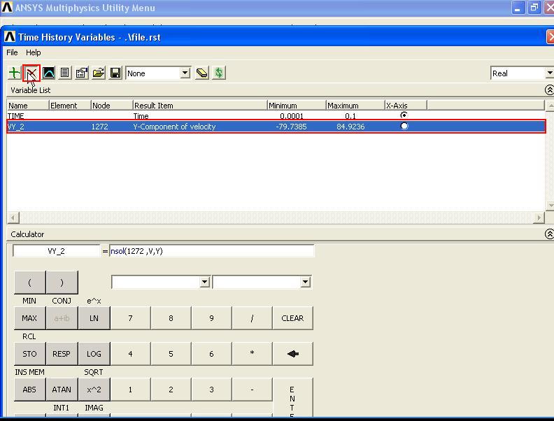
Add Time-History Variable window appears. From Nodal Solution click Velocity Solution - Y-Component of velocity and click OK.

Node for Data window appears. Pick left bottom corner of bracket as shown in the figure and click OK.

In Time History Variables window click once on VY_2 (Y-Component of velocity) and click on Graph Data button.


Acceleration Graph: From Main Menu click TimeHist Postpro - Variable Viewer.

Time History Variables window appears. Delete VY_2(Y-Component of velocity) from list.
Then click on Add Data button.

Add Time-History Variable window appears. From Nodal Solution click Acceleration Solution - Y-Component of acceleration and click OK.

Node for Data window appears. Pick left bottom corner of bracket as shown in the figure and click OK.

In Time History Variables window click once on AY_2 (Y-Component of acceleration) and click on Graph Data button.


============================================================
============================================================
Exercise 2: Transient Analysis of a Beam
Transient dynamic analysis is a technique used to determine the dynamic response of a structure under a time-varying load. The time frame for this type of analysis is such that inertia or damping effects of the structure are considered to be important. Cases where such effects play a major role are under step or impulse loading conditions, for example, where there is a sharp load change in a fraction of time. If inertia effects are negligible for the loading conditions being considered, a static analysis may be used instead.
Transient dynamic analysis is a technique used to determine the dynamic response of a structure under a time-varying load. The time frame for this type of analysis is such that inertia or damping effects of the structure are considered to be important. Cases where such effects play a major role are under step or impulse loading conditions, for example, where there is a sharp load change in a fraction of time. If inertia effects are negligible for the loading conditions being considered, a static analysis may be used instead.
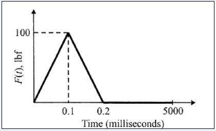
In this example, a beam is constrained at two end. And its cross section is square with side of 1 inch. A 100 pound force in 0.1 millisecond is applied to the center of the beam. The aim is to produce a graph of Displacement, Velocity, Acceleration of middle point of beam in terms of time.

At this time the amount of force is zero as shown in figure.

1). To define Element Type, from Main Menu click Preprocessor - Element Type - Add/Edit/Delete. Element Types window appears. Then click on Add button. Library of Element Types window appears. From left column select Beam and from right column select 2D elastic 3 and click OK.

BEAM3 is added to the Element Types window. Close this window.

2). To define Element Properties, from Main Menu click Preprocessor - Real Constants - Add/Edit/Delete. Real Constants window appears. Click on Add button. Type 1 BEAM3 is added to the window. Click OK.

Real Constants for BEAM3 window appears. In Cross-sectional area box enter 1 inch^2. In Area moment of inertia box enter 1/12. In Total beam height box enter 1 and click OK.

Set 1 is added to the Real Constants window. Close this window.

3). To define Material Properties, from Main Menu click Preprocessor - Material Props - Material Models. Define Material Model Behavior window appears. Select Structural - Linear - Elastic - Isotropic. Enter EX = 29e6 and PRXY = 0.3 and click OK.

To define Density, in Define Material Model Behavior window, click Structural - Density. Enter DENS = 0.2836 and click OK.

Close Define Material Model Behavior window.

4). To create the Geometry, from Main Menu click Preprocessor - Modeling - Create - Keypoints - In Active CS. Create the following points: 1.(-18,0,0) - 2.(18,0,0) and click OK.


In next stage, the points must be connected together. From Main Menu click Preprocessor - Modeling - Create - Lines - Lines - In Active Coord. Lines in Active Coord window appears. Pick these two points and click OK.

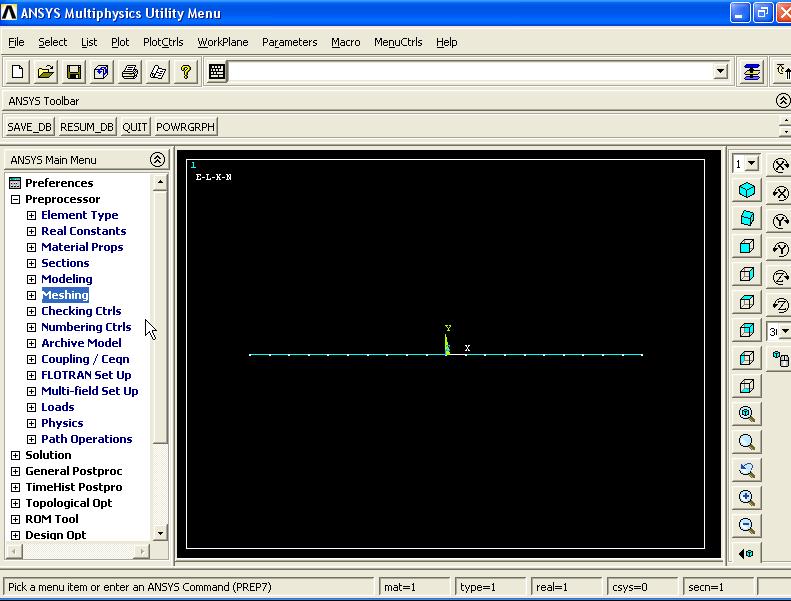
5). To Mesh the model, from Main Menu click Preprocessor - Meshing - Size Cntrls - ManualSize - Lines - All Lines. Element Sizes on All Selected Lines window appears. In No. of element divisions box enter 20 and click OK.

Then from Main Menu click Preprocessor - Meshing - Mesh - Lines. Mesh Lines window appears. Pick the line and click OK.

To display the nodes, from Menu click Plot - Multi-Plots.

To view the node numbers, from Menu click PlotCtrls - Numbering... Plot Numbering Controls window appears. Select Node numbers option and click OK.


===========================================================
Transient Analysis Stage:
6). From Main Menu click Solution - Analysis Type - New Analysis. New Analysis window appears. Select Transient option and click OK.

Transient Analysis window appears. Select Full option and click OK.

7). To apply Boundary Conditions, from Main Menu click Preprocessor - Loads - Define Loads - Apply - Structural - Displacement - On Nodes. Apply U, ROT on Nodes window appears. Pick both end nodes and click OK.

Apply U, ROT on Nodes window appears. From list select All DOF option and click OK.

8). To apply the Force, from Main Menu click Preprocessor - Loads - Define Loads - Apply - Structural - Force/Moment - On Nodes. Apply F/M on Nodes window appears. Pick the node number 12 and click OK.

Apply F/M on Nodes window appears. From first list select FY and in Force/moment value box enter -100 and click OK.


===========================================================
Transient Analysis Stage:
We want to solve the problem in three steps. This is done according to the F(t) graph. The 3 steps are based on time interval of: 1.(0 - 0.1 milliseconds) - 2.(0.1 - 0.2) - 3.(0.2 - 5seconds). Each step is called Load step.

Step 1: From Main Menu click Solution - Analysis Type - Sol'n Controls - Solution Controls window appears. In Basic tab, enter 1e-4s in Time at end of load step box. In Number of substeps box enter 20. In Max no. of substeps box enter 0 and In Min no. of substeps box enter 20. Select All solution items option. From Frequency: list select Write every substep.

Enter Transient tab in Solution Controls window. Select Ramped loading option. In Stiffness matrix multiplier (BETA) box enter 0.005 and click OK.

Now the information related to the first step of loading must be saved. To do this, from Main Menu click Solution - Load Step Opts - Write LS File. Write Load Step File window appears. In Load step file number box enter 1 and click OK.

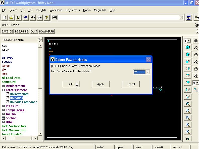
Step 2: For the second loading step in which the applied load reached 0, we must delete the applied load to the middle node. To do this from Main Menu click Solution - Define Loads - Delete - Structural - Force/Moment - On Nodes. Delete F/M on Nodes window appears. Pick the middle node and click OK.

Delete F/M on Nodes window appears. From list select FY and click OK.

From Main Menu click Solution - Analysis Type - Sol'n Controls - Solution Controls window appears. In Basic tab, in Time at end of loadstep box enter 2e-4s and click OK.

Now the information related to the second step of loading must be saved. To do this, from Main Menu click Solution - Load Step Opts - Write LS File. Write Load Step File window appears. In Load step file number box enter 2 and click OK.

Step 3: For the third loading step, from Main Menu click Solution - Analysis Type - Sol'n Controls - Solution Controls window appears. In Basic tab, in Time at end of loadstep box enter 0.5s. In Number of substeps box enter 200. In Max no. of substeps box enter 0 and In Min no. of substeps box enter 200. Click OK.

Now the information related to the second step of loading must be saved. To do this, from Main Menu click Solution - Load Step Opts - Write LS File. Write Load Step File window appears. In Load step file number box enter 3 and click OK.

===========================================================
Solution Stage:
From Main Menu click Solution - Solve - From LS Files.

Solved Load Step Files window appears. In Starting LS file number box enter 1 and in Ending LS file number box enter 3 and click OK.

Note window appears. Close the window.

===========================================================
Displacement Graph: From Main Menu click TimeHist Postpro. Time History Variables window appears. Click on Add Data button.

Add Time-History Variable window appears. From Nodal Solution click DOF Solution - Y-Component of displacement and click OK.

Node for Data window appears. Pick the middle point and click OK.

In Time History Variables window click once on UY_2 (Y-Component of displacement) then click on Graph Data button.


Velocity Graph: From Main Menu click TimeHist Postpro - Variable Viewer.

Time History Variables window appears. Delete UY_2(Y-Component of displacement) from list.

Then click on Add Data button.

Add Time-History Variable window appears. From Nodal Solution click Velocity Solution - Y-Component of velocity and click OK.

Node for Data window appears. Pick the middle points and click OK.

In Time History Variables window click once on VY_2 (Y-Component of velocity) and click on Graph Data button.


Acceleration Graph: From Main Menu click TimeHist Postpro - Variable Viewer.

Time History Variables window appears. Delete VY_2(Y-Component of velocity) from list.

Then click on Add Data button.

Add Time-History Variable window appears. From Nodal Solution click Acceleration Solution - Y-Component of acceleration and click OK.

Node for Data window appears. Pick the middle points (12) and click OK.

In Time History Variables window click once on AY_2 (Y-Component of acceleration) and click on Graph Data button.


BEAM3 is added to the Element Types window. Close this window.

2). To define Element Properties, from Main Menu click Preprocessor - Real Constants - Add/Edit/Delete. Real Constants window appears. Click on Add button. Type 1 BEAM3 is added to the window. Click OK.

Real Constants for BEAM3 window appears. In Cross-sectional area box enter 1 inch^2. In Area moment of inertia box enter 1/12. In Total beam height box enter 1 and click OK.

Set 1 is added to the Real Constants window. Close this window.

3). To define Material Properties, from Main Menu click Preprocessor - Material Props - Material Models. Define Material Model Behavior window appears. Select Structural - Linear - Elastic - Isotropic. Enter EX = 29e6 and PRXY = 0.3 and click OK.

To define Density, in Define Material Model Behavior window, click Structural - Density. Enter DENS = 0.2836 and click OK.

Close Define Material Model Behavior window.

4). To create the Geometry, from Main Menu click Preprocessor - Modeling - Create - Keypoints - In Active CS. Create the following points: 1.(-18,0,0) - 2.(18,0,0) and click OK.


In next stage, the points must be connected together. From Main Menu click Preprocessor - Modeling - Create - Lines - Lines - In Active Coord. Lines in Active Coord window appears. Pick these two points and click OK.

5). To Mesh the model, from Main Menu click Preprocessor - Meshing - Size Cntrls - ManualSize - Lines - All Lines. Element Sizes on All Selected Lines window appears. In No. of element divisions box enter 20 and click OK.

Then from Main Menu click Preprocessor - Meshing - Mesh - Lines. Mesh Lines window appears. Pick the line and click OK.

To display the nodes, from Menu click Plot - Multi-Plots.
To view the node numbers, from Menu click PlotCtrls - Numbering... Plot Numbering Controls window appears. Select Node numbers option and click OK.


===========================================================
Transient Analysis Stage:
6). From Main Menu click Solution - Analysis Type - New Analysis. New Analysis window appears. Select Transient option and click OK.
Transient Analysis window appears. Select Full option and click OK.
7). To apply Boundary Conditions, from Main Menu click Preprocessor - Loads - Define Loads - Apply - Structural - Displacement - On Nodes. Apply U, ROT on Nodes window appears. Pick both end nodes and click OK.

Apply U, ROT on Nodes window appears. From list select All DOF option and click OK.

8). To apply the Force, from Main Menu click Preprocessor - Loads - Define Loads - Apply - Structural - Force/Moment - On Nodes. Apply F/M on Nodes window appears. Pick the node number 12 and click OK.

Apply F/M on Nodes window appears. From first list select FY and in Force/moment value box enter -100 and click OK.


===========================================================
Transient Analysis Stage:
We want to solve the problem in three steps. This is done according to the F(t) graph. The 3 steps are based on time interval of: 1.(0 - 0.1 milliseconds) - 2.(0.1 - 0.2) - 3.(0.2 - 5seconds). Each step is called Load step.
Step 1: From Main Menu click Solution - Analysis Type - Sol'n Controls - Solution Controls window appears. In Basic tab, enter 1e-4s in Time at end of load step box. In Number of substeps box enter 20. In Max no. of substeps box enter 0 and In Min no. of substeps box enter 20. Select All solution items option. From Frequency: list select Write every substep.

Enter Transient tab in Solution Controls window. Select Ramped loading option. In Stiffness matrix multiplier (BETA) box enter 0.005 and click OK.

Now the information related to the first step of loading must be saved. To do this, from Main Menu click Solution - Load Step Opts - Write LS File. Write Load Step File window appears. In Load step file number box enter 1 and click OK.

Step 2: For the second loading step in which the applied load reached 0, we must delete the applied load to the middle node. To do this from Main Menu click Solution - Define Loads - Delete - Structural - Force/Moment - On Nodes. Delete F/M on Nodes window appears. Pick the middle node and click OK.

Delete F/M on Nodes window appears. From list select FY and click OK.
From Main Menu click Solution - Analysis Type - Sol'n Controls - Solution Controls window appears. In Basic tab, in Time at end of loadstep box enter 2e-4s and click OK.

Now the information related to the second step of loading must be saved. To do this, from Main Menu click Solution - Load Step Opts - Write LS File. Write Load Step File window appears. In Load step file number box enter 2 and click OK.

Step 3: For the third loading step, from Main Menu click Solution - Analysis Type - Sol'n Controls - Solution Controls window appears. In Basic tab, in Time at end of loadstep box enter 0.5s. In Number of substeps box enter 200. In Max no. of substeps box enter 0 and In Min no. of substeps box enter 200. Click OK.

Now the information related to the second step of loading must be saved. To do this, from Main Menu click Solution - Load Step Opts - Write LS File. Write Load Step File window appears. In Load step file number box enter 3 and click OK.

===========================================================
Solution Stage:
From Main Menu click Solution - Solve - From LS Files.

Solved Load Step Files window appears. In Starting LS file number box enter 1 and in Ending LS file number box enter 3 and click OK.

Note window appears. Close the window.

===========================================================
Displacement Graph: From Main Menu click TimeHist Postpro. Time History Variables window appears. Click on Add Data button.

Add Time-History Variable window appears. From Nodal Solution click DOF Solution - Y-Component of displacement and click OK.
Node for Data window appears. Pick the middle point and click OK.

In Time History Variables window click once on UY_2 (Y-Component of displacement) then click on Graph Data button.


Velocity Graph: From Main Menu click TimeHist Postpro - Variable Viewer.

Time History Variables window appears. Delete UY_2(Y-Component of displacement) from list.

Then click on Add Data button.
Add Time-History Variable window appears. From Nodal Solution click Velocity Solution - Y-Component of velocity and click OK.
Node for Data window appears. Pick the middle points and click OK.

In Time History Variables window click once on VY_2 (Y-Component of velocity) and click on Graph Data button.


Acceleration Graph: From Main Menu click TimeHist Postpro - Variable Viewer.

Time History Variables window appears. Delete VY_2(Y-Component of velocity) from list.

Then click on Add Data button.
Add Time-History Variable window appears. From Nodal Solution click Acceleration Solution - Y-Component of acceleration and click OK.
Node for Data window appears. Pick the middle points (12) and click OK.

In Time History Variables window click once on AY_2 (Y-Component of acceleration) and click on Graph Data button.


==========================================================
Exercise 3: Dynamic Simulation of the Universal Joint
In this exercise, we'll perform a dynamics simulation for the assembly created in Exercise 11. The assembly is entirely made of steel, which is the default material used in .
We assume a hinge set up at the top of the upper yoke, such that the whole assembly can swing in the XY plane and behaves like a double-pendulum [1]. Initially, the lower yoke is raised to form an angle of 30 degrees with the vertical axis, and then released [2]. The only external force, other than the reaction forces at the hinge, acting on the assembly is the gravitational force. We want to observe the double-pendulum behavior of the assembly.
Since our concern is the double-pendulum behavior of the assembly, the body deformation can be neglected. Therefore, we assume all bodies are rigid. We'll use a built-in system in the Workbench, called Dynamics>, which assumes all bodies are rigid and has capabilities of performing rigid-body dynamic simulations. We'll further assume that the combination of the swivel, four bushings, and four pins is an integrated part, i.e., they are bonded together. This assumption should be reasonable as long as the double-pendulum behavior is the only concern. This assumption not only simplifies the model setup in but also reduces computation time.


Nice article, thank you for sharing wonderful information. I am happy to find your blog on the internet.
ReplyDeleteYou can also check - Ansys Training in India
Nice article, thank you for sharing wonderful information. I am happy to find your blog on the internet.
ReplyDeleteYou can also check - Best Ansys Course In India