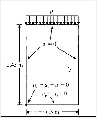
Eigenvalue Buckling of a steel plate: The model is a shell steel plate with thickness of the 3mm. This plate is fixed at one end in the ground. A uniform Pressure (P) is applied to the top of the plate. The aim is to find the maximum allowable pressure P that prevents buckling.
1). To define Element Type, from Main menu click Preprocessor - Element Type - Add/Edit/Delete. Element Types window appears. Click on Add button. Library of Element Types window appears. From left column select Shell and from right column select Elastic 4node 63 and click OK.

SHELL63 is added to the Element Types window. Close the window.

2). To define Element Properties, from Main Menu click Preprocessor - Real Constants - Add/Edit/Delete. Real Constants window appears. Click on Add button. Click OK.

Real Constant Set Number 1, for SHELL63 window appears. In Shell thickness at node I box enter 0.003mm and click OK. Close Real Constants window.

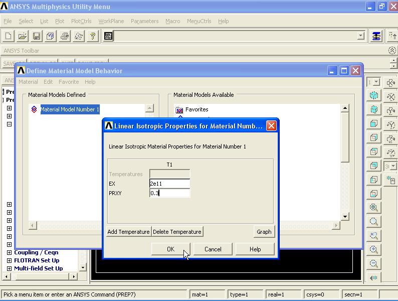
3). To define Material Properties, from Main Menu click Preprocessor - Material Props - Material Models. Define Material Model Behavior window appears. Click Structural - Linear - Elastic - Isotropic. Enter EX = 2e11 and PRXY = 0.3 and click OK.
4). To create the Geometry, from Main Menu click Preprocessor - Modeling - Create - Areas - Rectangle - By Dimensions. Create Rectangle by Dimensions window appears. Enter X1 = 0, X2 = 0.3, Y1 = 0, and Y2 = 0.45 and click OK.


5). Before meshing we need to display the line numbers. From Menu click PlotCtrls - Numbering. Plot Numbering Controls window appears. Activate Line numbers and click OK.


Then from Menu click Plot - Lines.

To mesh the model from Main Menu click Preprocessor - Meshing - Size Cntrls - ManualSize - Lines - Picked Lines. Then pick lines 1 and 3 and click OK.

Element Sizes on Picked Lines window appears. In No. of element divisions box enter 15 and click OK.

Repeat the process again for the other two lines. From Main Menu click Preprocessor - Meshing - Size Cntrls - ManualSize - Lines - Picked Lines. Then pick lines 2 and 4 and click OK.

Element Sizes on Picked Lines window appears. In No. of element divisions box enter 25 and click OK.

From Main Menu click Preprocessor - Meshing - Mesh - Areas - Mapped - 3 or 4 sided. Mesh Areas window appears. Pick the area and click OK.


6). To apply Boundary Conditions from Main Menu click Preprocessor - Loads - Define Loads - Apply - Structural - Displacement - On Nodes. Apply U, ROT on Nodes window appears. Then select Box option from window and select the top, bottom, left and right edges nodes. Click OK.

Apply U, ROT on Nodes window appears. From list select UZ and click OK.

From Main Menu click Preprocessor - Loads - Define Loads - Apply - Structural - Displacement - On Nodes. Apply U, ROT on Nodes window appears. Then select Box option from window and select the bottom edge nodes. Click OK.

Apply U, ROT on Nodes window appears. From list select UY and click OK.

From Main Menu click Preprocessor - Loads - Define Loads - Apply - Structural - Displacement - On Nodes. Apply U, ROT on Nodes window appears. Pick the bottom left corner node. Click OK.

Apply U, ROT on Nodes window appears. From list select UX and click OK.

7). To apply Pressure, from Main Menu click Preprocessor - Loads - Define Loads - Apply - Structural - Pressure - On Nodes. Apply PRES on Nodes window appears. Select Box option from the window and select all the top edge nodes. Click OK.

Apply PRES on Nodes window appears. In Load PRES value box enter 1. Click OK.

8). To define Analysis Type, from Main Menu click Solution - Analysis Type - New Analysis - New Analysis window appears. Select static option and click OK.

Then from Main Menu click Solution - Analysis Type - Sol'n Controls. Solution Controls window appears. In Basic tab, select Calculate prestress effects option and click OK.

===========================================================
Static Solution Stage:
From Main Menu click Solution - Solve - Current LS. Click OK to solve the problem. Close the window.

Finally from Main Menu click on Finish.

===========================================================
Buckling Analysis:
From Main Menu click Solution - Analysis Type - New Analysis. New Analysis window appears. From list select Eigen Buckling and click OK.

From Main Menu click Solution - Analysis Type - Analysis Options. Eigenvalue Buckling Options window appears. In No. of modes to extract box enter 4 and click OK.

From Main Menu click Solution - Load Step Opts - ExpansionPass - Single Expand - Expand Modes. Expand Modes window appears. In No. of modes to expand box enter 4 and click OK.

Again solve the problem. From Main Menu click Solution - Solve - Current LS. Click OK to start solution.

Post processing Stage:
From Main Menu click General Postproc - List Results - Detailed Summary. SET, LIST Command window appears. The 4 loads are the critical loads in 4 modes. Buckling always happen in first mode. It means that the buckling critical load is 0.23464E+06 MPa.

to view the first mode shape, from Main Menu click General Postproc - Read Results - First Set.

Then from Main Menu click General Postproc - Plot Results - Deformed Shape. Plot Deformed Shape window appears. Click OK.


To animate the deformation, from Menu click PlotCtrls - Animate - Mode Shape. Animate Mode Shape window appears. From left column select DOF Solution and from right column select Def + undeformed option and click OK.


From Main Menu click General Postproc - Plot Results - Contour Plot - Nodal Solu. Contour Nodal Solution Data window appears. Select DOF Solution - Displacement vector sum. Click OK.


Shape mode 2:
From Main Menu click General Postproc - Read Results - Next Set.

Then from Main Menu click General Postproc - Plot Results - Contour Plot - Nodal Solu. Contour Nodal Solution Data window appears. Click DOF Solution - Displacement vector sum. Click OK.


==========================================================
Eigenvalue Buckling Analysis of a Beam:
In science, buckling is a mathematical instability, leading to a failure mode. Theoretically, buckling is caused by a bifurcation in the solution to the equations of static equilibrium. At a certain stage under an increasing load, further load is able to be sustained in one of two states of equilibrium: an undeformed state or a laterally-deformed state. In practice, buckling is characterized by a sudden failure of a structural member subjected to high compressive stress, where the actual compressive stress at the point of failure is less than the ultimate compressive stresses that the material is capable of withstanding. Mathematical analysis of buckling makes use of an axial load eccentricity that introduces a moment, which does not form part of the primary forces to which the member is subjected. When load is constantly being applied on a member, such as column, it will ultimately become large enough to cause the member to become unstable. Further load will cause significant and somewhat unpredictable deformations, possibly leading to complete loss of load-carrying capacity. The member is said to have buckled, to have deformed.
Buckling loads are critical loads where certain types of structures become unstable. Each load has an associated buckled mode shape; this is the shape that the structure assumes in a buckled condition.
Buckling loads are critical loads where certain types of structures become unstable. Each load has an associated buckled mode shape; this is the shape that the structure assumes in a buckled condition.
- Eigenvalue: Eigenvalue buckling analysis predicts the theoretical buckling strength of an ideal elastic structure. It computes the structural eigenvalues for the given system loading and constraints. This is known as classical Euler buckling analysis. Buckling loads for several configurations are readily available from tabulated solutions. However, in real-life, structural imperfections and non-linearities prevent most real-world structures from reaching their eigenvalue predicted buckling strength; ie. it over-predicts the expected buckling loads. This method is not recommended for accurate, real-world buckling prediction analysis
A column is fixed at one end and its length is 100mm. And its cross section is square with side of 10mm. This column is under a compressive axial pressure (P). The aim is to find Buckling critical loads.

1). To define Element Types, from Main Menu click Preprocessor - Element Type - Add/Edit/Delete. Element Types window appears. Click on Add button. Library of Element Types window appears. From left column select Beam and from right column select 2D elastic 3 and click OK.

BEAM3 is added to the Element Types window. Close the window.

2). To define Element Properties, from Main Menu click Preprocessor - Real Constants - Add/Edit/Delete. Real Constants window appears. Click on Add button. Click OK.

Real Constants for BEAM3 window appears. In Cross-sectional area box enter 100 and in Area moment of inertia box enter 833.33 and in Total beam height box enter 10 and click OK. Close Real Constants window.

3). To define Material Properties, from Main Menu click Preprocessor - Material Props - Material Models. Define Material Model Behavior window appears. Click Structural - Linear - Elastic - Isotropic. Enter EX = 2e5 and PRXY = 0.3 and click OK.

4). To create the Geometry, from Main Menu click Preprocessor - Modeling - Create - Keypoints - In Active CS. Create the following points: 1.(0,0,0) - 2.(0,100,0) and click OK.

Then the points must be connected. From Main Menu click Preprocessor - Modeling - Create - Lines - Lines - In Active Coord. Lines in Active Coord window appears. Connect point 1 to point 2 and click OK.

5). To Mesh the model, from Main Menu click Meshing - Size Cntrls - ManualSize - Lines - All Lines. Element Sizes on All Selected Lines window appears. In Element edge length box enter 10mm and click OK.


From Main Menu click Meshing - Mesh - Lines. Mesh Lines window appears. Pick the model and click OK.

6). To define Analysis Type, from Main Menu click Solution - Analysis Type - New Analysis. New Analysis window appears. Select Static option and click OK.

Then from Main Menu click Solution - Analysis Type - Sol'n Controls. Solution Controls window appears. In Basic tab, select Calculate prestress effects option and click OK.

7). To apply boundary conditions, from Main Menu click Preprocessor - Loads - Define Loads - Apply - Structural - Displacement - On Nodes. Apply U, ROT on Nodes window appears. Select the bottom node and click OK.

Apply U, ROT on Nodes window appears. From list select All DOF and click OK.

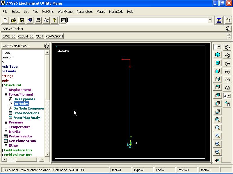
8). In Buckling analysis the load is always 1 unit. To apply loading, from Main Menu click Preprocessor - Loads - Define Loads - Apply - Structural - Force/Moment - On Nodes. Apply F/M on Nodes window appears. Pick the top node and click OK.

Apply F/M on Nodes window appears. From the list select FY and in Force/moment value box enter -1 and click OK.

Static Solution Stage:
From Main Menu click Solution - Solve - Current LS. Click OK to start solution. Close the window.

Then from Main Menu click Finish.

Buckling Analysis Stage:
In next stage, we will carry out the Buckling analysis. From Main Menu click Solution - Analysis Type - New Analysis. New Analysis window appears. From list select Eigen Buckling and click OK.

Then from Main Menu click Solution - Analysis Type - Analysis Options. Eigenvalue Buckling Options window appears. In No. of modes to extract box enter 4 and click OK.

Then solve the problem again. From Main Menu click Solution - Solve - Current LS. Click OK to start solution. Close the window.

Then from Main Menu click Finish.

From Main Menu click Solution - Analysis Type - ExpansionPass. Expansion Pass window appears. Activate Expansion Pass and click OK.

From Main Menu click Solution - Load Step Opts - ExpansionPass - Single Expand - Expand Modes. Expand Modes window appears. In No. of modes to expand box enter 4 and click OK.

Solve the problem again. From Main Menu click Solution - Solve - Current LS. Click OK to start solution. Close the window.

Post Processing Stage:
Now the solution stage is ended, and the results can be extracted. From Main Menu click General Postproc - List Results - Detailed Summary. SET, LIST Command table appears. The left column displays the critical loads in 4 modes.

NOTE: In practice buckling always happen in first mode. The buckling load is 41123 N. To view the displacement shape of the first mode, from Main Menu click General Postproc - Read Results - First Set.

Then from Main Menu click General Postproc - Plot Results - Deformed Shape. Plot Deformed Shape window appears. Select Def + undeformed option and click OK.

Mode 1 shape:

To view the displacement shape of the mode 2, from Main Menu click General Postproc - Read Results - Next Set.

Then from Main Menu click General Postproc - Plot Results - Deformed Shape. Plot Deformed Shape window appears. Select Def + undeformed option and click OK.

Mode 2 shape:

To view the displacement shape of the mode 3, from Main Menu click General Postproc - Read Results - Next Set.

Then from Main Menu click General Postproc - Plot Results - Deformed Shape. Plot Deformed Shape window appears. Select Def + undeformed option and click OK.

Mode 3 shape:

To animate the displacement, from Menu click PlotCtrls - Animate - Mode Shape...

Animate Mode Shape window appears. From left column select DOF solution and from right column select Def + undeformed option and click OK.


==========================================================
==========================================================
Non-linear Buckling Analysis of a Beam:

1). To define Element Types, from Main Menu click Preprocessor - Element Type - Add/Edit/Delete. Element Types window appears. Click on Add button. Library of Element Types window appears. From left column select Beam and from right column select 2D elastic 3 and click OK.

BEAM3 is added to the Element Types window. Close the window.

2). To define Element Properties, from Main Menu click Preprocessor - Real Constants - Add/Edit/Delete. Real Constants window appears. Click on Add button. Click OK.

Real Constants for BEAM3 window appears. In Cross-sectional area box enter 100 and in Area moment of inertia box enter 833.33 and in Total beam height box enter 10 and click OK. Close Real Constants window.

3). To define Material Properties, from Main Menu click Preprocessor - Material Props - Material Models. Define Material Model Behavior window appears. Click Structural - Linear - Elastic - Isotropic. Enter EX = 2e5 and PRXY = 0.3 and click OK.

4). To create the Geometry, from Main Menu click Preprocessor - Modeling - Create - Keypoints - In Active CS. Create the following points: 1.(0,0,0) - 2.(0,100,0) and click OK.

Then the points must be connected. From Main Menu click Preprocessor - Modeling - Create - Lines - Lines - In Active Coord. Lines in Active Coord window appears. Connect point 1 to point 2 and click OK.

5). To Mesh the model, from Main Menu click Meshing - Size Cntrls - ManualSize - Lines - All Lines. Element Sizes on All Selected Lines window appears. In Element edge length box enter 1mm and click OK.


From Main Menu click Meshing - Mesh - Lines. Mesh Lines window appears. Pick the model and click OK.

To define Solution Type, from Main Menu click Solution - Analysis Type - New Analysis. New Analysis window appears. Select Static option and click OK.

Then from Main Menu click Solution - Analysis Type - Sol'n Controls. Solution Controls window appears. From Basic tab and in Analysis Options section, from menu select Large Displacement Static option. In Automatic time stepping list select On.
In Number of substeps box enter 20, in Max no. of substeps box enter 1000, and in Min no. of substeps box enter 1.

Then select Nonlinear tab from Solution Controls window. From Line search list select On and in Maximum number of iterations box enter 1000 and click OK.

6). To apply Boundary Conditions, from Main Menu click Preprocessor - Solution - Define Loads - Apply - Structural - Displacement - On Nodes. Apply U, ROT on Nodes window appears. Pick the bottom node and click OK.

Apply U, ROT on Nodes window appears. From list select All DOF and click OK.

7). To apply Loading, from Main Menu click Preprocessor - Solution - Define Loads - Apply - Structural - Force/Moment - On Nodes. Apply F/M on Nodes window appears. Pick the top node and click OK.

Apply F/M on Nodes window appears. From list select FY and for the force value enter -50000 N. Click Apply.

The role of the force in X direction is to make the structure unstable. To apply a force in X direction, again pick the top node and click OK.

Apply F/M on Nodes window appears. From list select FX and for force value enter -250N and click OK. This horizontal load will persuade the beam to buckle at the minimum buckling load.

 =============================================================
Solution Stage:
From Main Menu click Solution - Solve - Current LS. Click OK to start solution. Close the window.

From Menu click PlotCtrls - Style - Size and Shape.

Size and Shape window appears. Activate Display of element option and click OK.

 =============================================================
Post Processing Stage:
From Main Menu click General Postproc - Plot Results - Contour Plot - Nodal Solu. Contour Nodal Solution Data window appears. Click DOF Solution - X-Component of displacement. Click OK.


Y-Component of displacement:

Displacement vector sum:

To find the buckling critical load, from Main Menu click TimeHist Postpro. Time History Variables window appears. Click on Add Data button at top left side of the window.

Add Time-History Variable window appears. Click Nodal Solution - DOF Solution - Y-Component of displacement. Click OK.

Node for Data window appears. Pick the top node and click OK.

From Time History Variables window, again click on Add Data button at top left side of the window. Add Time-History Variable window appears. Click Reaction Forces - Structural Forces - Y-Component of force. Click OK.

Node for Data window appears. Then pick the bottom node and click OK.


In the Time History Variables window, from X-Axis column select the option for Y-Component of force.

Then from window, select Y-Component of displacement.

Then click on Graph Data button to view the graph.

The plot shows how the beam became unstable and buckled with a load of approximately 40,000 N, the point where a large deflection occurred due to a small increase in force. This is slightly less than the eigen-value solution of 41,123 N, which was expected due to non-linear geometry issues discussed above.
 Buckling in ANSYS:
==========================================================
Non-linear Buckling Analysis of a Beam:
In science, buckling is a mathematical instability, leading to a failure mode. Theoretically, buckling is caused by a bifurcation in the solution to the equations of static equilibrium. At a certain stage under an increasing load, further load is able to be sustained in one of two states of equilibrium: an undeformed state or a laterally-deformed state. In practice, buckling is characterized by a sudden failure of a structural member subjected to high compressive stress, where the actual compressive stress at the point of failure is less than the ultimate compressive stresses that the material is capable of withstanding. Mathematical analysis of buckling makes use of an axial load eccentricity that introduces a moment, which does not form part of the primary forces to which the member is subjected. When load is constantly being applied on a member, such as column, it will ultimately become large enough to cause the member to become unstable. Further load will cause significant and somewhat unpredictable deformations, possibly leading to complete loss of load-carrying capacity. The member is said to have buckled, to have deformed.
Buckling loads are critical loads where certain types of structures become unstable. Each load has an associated buckled mode shape; this is the shape that the structure assumes in a buckled condition.
Buckling loads are critical loads where certain types of structures become unstable. Each load has an associated buckled mode shape; this is the shape that the structure assumes in a buckled condition.
Non-linear: Non-linear buckling analysis is more accurate than eigenvalue analysis because it employs non-linear, large-deflection, static analysis to predict buckling loads. Its mode of operation is very simple: it gradually increases the applied load until a load level is found whereby the structure becomes unstable (ie. suddenly a very small increase in the load will cause very large deflections). The true non-linear nature of this analysis thus permits the modeling of geometric imperfections, load perturbations, material nonlinearities and gaps. For this type of analysis, note that small off-axis loads are necessary to initiate the desired buckling mode.
A column is fixed at one end and its length is 100mm. And its cross section is square with side of 10mm. This column is under a compressive axial pressure (P). The aim is to find Buckling critical loads.

1). To define Element Types, from Main Menu click Preprocessor - Element Type - Add/Edit/Delete. Element Types window appears. Click on Add button. Library of Element Types window appears. From left column select Beam and from right column select 2D elastic 3 and click OK.
BEAM3 is added to the Element Types window. Close the window.
2). To define Element Properties, from Main Menu click Preprocessor - Real Constants - Add/Edit/Delete. Real Constants window appears. Click on Add button. Click OK.
Real Constants for BEAM3 window appears. In Cross-sectional area box enter 100 and in Area moment of inertia box enter 833.33 and in Total beam height box enter 10 and click OK. Close Real Constants window.
3). To define Material Properties, from Main Menu click Preprocessor - Material Props - Material Models. Define Material Model Behavior window appears. Click Structural - Linear - Elastic - Isotropic. Enter EX = 2e5 and PRXY = 0.3 and click OK.
4). To create the Geometry, from Main Menu click Preprocessor - Modeling - Create - Keypoints - In Active CS. Create the following points: 1.(0,0,0) - 2.(0,100,0) and click OK.
Then the points must be connected. From Main Menu click Preprocessor - Modeling - Create - Lines - Lines - In Active Coord. Lines in Active Coord window appears. Connect point 1 to point 2 and click OK.
5). To Mesh the model, from Main Menu click Meshing - Size Cntrls - ManualSize - Lines - All Lines. Element Sizes on All Selected Lines window appears. In Element edge length box enter 1mm and click OK.

To define Solution Type, from Main Menu click Solution - Analysis Type - New Analysis. New Analysis window appears. Select Static option and click OK.

Then from Main Menu click Solution - Analysis Type - Sol'n Controls. Solution Controls window appears. From Basic tab and in Analysis Options section, from menu select Large Displacement Static option. In Automatic time stepping list select On.
In Number of substeps box enter 20, in Max no. of substeps box enter 1000, and in Min no. of substeps box enter 1.

Then select Nonlinear tab from Solution Controls window. From Line search list select On and in Maximum number of iterations box enter 1000 and click OK.

6). To apply Boundary Conditions, from Main Menu click Preprocessor - Solution - Define Loads - Apply - Structural - Displacement - On Nodes. Apply U, ROT on Nodes window appears. Pick the bottom node and click OK.

Apply U, ROT on Nodes window appears. From list select All DOF and click OK.

7). To apply Loading, from Main Menu click Preprocessor - Solution - Define Loads - Apply - Structural - Force/Moment - On Nodes. Apply F/M on Nodes window appears. Pick the top node and click OK.

Apply F/M on Nodes window appears. From list select FY and for the force value enter -50000 N. Click Apply.

The role of the force in X direction is to make the structure unstable. To apply a force in X direction, again pick the top node and click OK.

Apply F/M on Nodes window appears. From list select FX and for force value enter -250N and click OK. This horizontal load will persuade the beam to buckle at the minimum buckling load.

Solution Stage:
From Main Menu click Solution - Solve - Current LS. Click OK to start solution. Close the window.

From Menu click PlotCtrls - Style - Size and Shape.

Size and Shape window appears. Activate Display of element option and click OK.


Post Processing Stage:
From Main Menu click General Postproc - Plot Results - Contour Plot - Nodal Solu. Contour Nodal Solution Data window appears. Click DOF Solution - X-Component of displacement. Click OK.


Y-Component of displacement:

Displacement vector sum:

To find the buckling critical load, from Main Menu click TimeHist Postpro. Time History Variables window appears. Click on Add Data button at top left side of the window.

Add Time-History Variable window appears. Click Nodal Solution - DOF Solution - Y-Component of displacement. Click OK.

Node for Data window appears. Pick the top node and click OK.

From Time History Variables window, again click on Add Data button at top left side of the window. Add Time-History Variable window appears. Click Reaction Forces - Structural Forces - Y-Component of force. Click OK.

Node for Data window appears. Then pick the bottom node and click OK.


In the Time History Variables window, from X-Axis column select the option for Y-Component of force.

Then from window, select Y-Component of displacement.

Then click on Graph Data button to view the graph.

The plot shows how the beam became unstable and buckled with a load of approximately 40,000 N, the point where a large deflection occurred due to a small increase in force. This is slightly less than the eigen-value solution of 41,123 N, which was expected due to non-linear geometry issues discussed above.

==========================================================
==========================================================
==========================================================
In science, buckling is a mathematical instability, leading to a failure mode. Theoretically, buckling is caused by a bifurcation in the solution to the equations of static equilibrium. At a certain stage under an increasing load, further load is able to be sustained in one of two states of equilibrium: an undeformed state or a laterally-deformed state. In practice, buckling is characterized by a sudden failure of a structural member subjected to high compressive stress, where the actual compressive stress at the point of failure is less than the ultimate compressive stresses that the material is capable of withstanding. Mathematical analysis of buckling makes use of an axial load eccentricity that introduces a moment, which does not form part of the primary forces to which the member is subjected. When load is constantly being applied on a member, such as column, it will ultimately become large enough to cause the member to become unstable. Further load will cause significant and somewhat unpredictable deformations, possibly leading to complete loss of load-carrying capacity. The member is said to have buckled, to have deformed.
Buckling loads are critical loads where certain types of structures become unstable. Each load has an associated buckled mode shape; this is the shape that the structure assumes in a buckled condition. There are two primary means to perform a buckling analysis:
Buckling loads are critical loads where certain types of structures become unstable. Each load has an associated buckled mode shape; this is the shape that the structure assumes in a buckled condition. There are two primary means to perform a buckling analysis:
- EigenvalueEigenvalue buckling analysis predicts the theoretical buckling strength of an ideal elastic structure. It computes the structural eigenvalues for the given system loading and constraints. This is known as classical Euler buckling analysis. Buckling loads for several configurations are readily available from tabulated solutions. However, in real-life, structural imperfections and nonlinearities prevent most real-world structures from reaching their eigenvalue predicted buckling strength; ie. it over-predicts the expected buckling loads. This method is not recommended for accurate, real-world buckling prediction analysis.
- Non-linearNon-linear buckling analysis is more accurate than eigenvalue analysis because it employs non-linear, large-deflection, static analysis to predict buckling loads. Its mode of operation is very simple: it gradually increases the applied load until a load level is found whereby the structure becomes unstable (i.e. suddenly a very small increase in the load will cause very large deflections). The true non-linear nature of this analysis thus permits the modeling of geometric imperfections, load perturbations, material nonlinearities and gaps. For this type of analysis, note that small off-axis loads are necessary to initiate the desired buckling mode.

After applying materials, creating the model and meshing, go to solution - Analysis type - New Analysis and select static.


Then click on Sol'n controls. Solution control window appears.

From basic tab check calculate prestress effects box and click OK. And then apply boundary conditions and load. The eigenvalue solver uses a unit force to determine the necessary buckling load. Applying a load other than 1 will scale the answer by a factor of the load.
After solving the problem in static mode, go to Solution - Analysis type - New Analysis then select Eigen Buckling option.

Then from Analysis type select Analysis Options. The Eigenvalue Analysis options appear.

Enter a value in No. of modes to extract (i.e. 4). Click on OK. And solve the problem again. After solution click on finish option. Then from Solution - Analysis Type - ExpansionPass - activate Expansion Pass.

Then, Solution - Load Step Opts - ExpansionPass - Single Expand - Expand modes. And enter the value of 4 in No. of modes to expand. Click OK. Again solve the problem.

Results: General Postproc - List Results - Detailed Summary.

To view the first mode, Read Results - First Set - then enter Plot results - Deformed Shape - Select Def + Undeformed - Click OK.

2). Nonlinear buckling analysis method: is more accurate than eigenvalue analysis because it employs non-linear, large-deflection, static analysis to predict buckling loads. Its mode of operation is very simple: it gradually increases the applied load until a load level is found whereby the structure becomes unstable (i.e. suddenly a very small increase in the load will cause very large deflections). The true non-linear nature of this analysis thus permits the modeling of geometric imperfections, load perturbations, material nonlinearities and gaps. For this type of analysis, note that small off-axis loads are necessary to initiate the desired buckling mode.
In this method, when commencing solution, the software gradually increase the applied load, up to a level, in which small increase in load will cause a big deformation.
All the element type, material selection, modeling and meshing is the same as above method. After this stages, enter Solution - Analysis type - New Analysis - Static - OK
Click Sol'n Controls - in solution controls select basic tab, then open Analysis Options menu, select Large Displacement Static - from Automatic time stepping select On, then, in Number of substeps box enter a value (20), in Max no. of substeps enter 1000, and in Min no. of substeps enter 1.

Then enter Nonlinear tab - From Line search select On option - from Maximum number of iterations enter 1000 - Click OK.

Next stage is applying boundary conditions and loading. When applying load, there are two loads one vertical and the other is horizontal (along X axis). The lateral is for making the structure unstable.

Then solve the problem.
To find critical loading of buckling, click on TimeHist Postpro,.

Click on Add Data button, then from Nodal solution select DOF Solution then select Y-Component of displacement. Click on OK.

Then in graphic area select the top node. Click OK.

Again, click on Add Data button. From reaction forces, structural forces, and select Y-component of force. Then select the lowest node point. From Time history variables, select Y-component of force. Then click on Graph Data button. The graph is produced.

=========================================================
Buckling analysis of a shell plate:

Element type: Shell - Elastic 4node 63 (SHELL63)
=======================================================
No comments:
Post a Comment