A steel plate with 1cm thickness and dimensions of 3m x 1m is shown. Through the holes, two pipes passes. All the system is in initial temperature of 25C. Then after a while a fluid with temperature of -35C flows through right hand side pipe and another fluid with temperature of 150C flows through left hand side pipe. The aim is to find the stresses in the plate which is created due to temperature variations in pipes. And also the deformation of the plate. Thermal conductivity of the plate is 40 W/m*C and thermal expansion coefficient is 12e-6.

1). From Menu click File - Change Jobname...

Change Jobname window appears. Enter Couple-Structural-Thermal for job name and click OK.

2). From Main Menu click Preferences. Preferences for GUI Filtering window appears. Select Thermal option and click OK.


4). To define properties of the element, from Main Menu click Preprocessor - Real Constants - Add/Edit/Delete. Real Constants window appears. Click on Add button


Apply U, ROT on Lines window appears. Select All DOF from list and click OK.

From Main Menu click Preprocessor - Loads - Define Loads - Apply - Structural - Temperature - From Therm Analy. Apply TEMP from Thermal Analysis window appears. Click on Browse button.

Select the file which was created at the beginning of the analysis (Couple-Structural-Thermal.rth) and click Open.

Apply TEMP from Thermal Analysis window again appears. Click on OK to close the window.

Next from Main Menu click Preprocessor - Loads - Define Loads - Settings - Reference Temp. Reference Temperature window appears. Enter 25C in Reference Temperature box and click OK.

===========================================================
Structural Solution Stage:
From Main Menu click Solution - Solve - Current LS. Click OK to start solution. Close the window.

===========================================================
Post Processing Stage:
From Main Menu click General Postproc - Plot Results - Contour Plot - Nodal Solu. Contour Nodal Solution Data window appears. From list click DOF Solution - X-Component of displacement. Click OK.


Y-Component of displacement:

Displacement vector sum:

Stress - X-Component of stress:

Y-Component of stress:

XY Shear stress:

Von mises stress:

To animate the deformation, from Menu click PlotCtrls - Animate - Mode Shape...

Animate Mode Shape window appears. From left column select Stress and from right column select von mises and click OK.

 ==========================================================
==========================================================


Change Jobname window appears. Enter Couple-Structural-Thermal for job name and click OK.

2). From Main Menu click Preferences. Preferences for GUI Filtering window appears. Select Thermal option and click OK.

3). To define Element Types, from Main Menu click Preprocessor - Element Type - Add/Edit/Delete. Element Types window appears. Click on Add button. Library of Element Types window appears. From left column select Solid and from right column select Quad 4node 55 and click OK.

PLANE55 is added to the Element Types window.

In this window click on Options button. PLANE55 element type options window appears. From Element behavior list select Plane Thickness option and click OK. Then close Element Types window.


Type 1 PLANE55 is added to the list. Click OK.

Real Constant Set Number 1, for PLANE55 window appears. In Z-Depth box enter 0.01m and click OK. Then close Real Constants window.

5). To define thermal properties of the material, from Main Menu click Preprocessor - Material Props - Material Models - Define Material Model Behavior window appears. Click Thermal - Conductivity - Isotropic. Enter KXX = 40 and click OK.

Close Define Material Model Behavior window.

6). To create the Geometry, from Main Menu click Preprocessor - Modeling - Create - Areas - Rectangle - By 2 Corners. Rectangle by 2 Corners window appears. Enter X = 0, Y = 0, Width = 3 and Height = 1m and click OK.


Then from Main Menu click Preprocessor - Modeling - Create - Areas - Circle - Solid Circle. Solid Circular Area window appears. Enter X = 0.75, Y = 0.5 and Radius = 0.25 and click Apply.


Again in Solid Circular Area window enter X = 2.25, Y = 0.5 and Radius = 0.25 and click OK.


Next we must subtract the areas of two circles from rectangle. From Main Menu click Preprocessor - Modeling - Operate - Booleans - Subtract - Areas. Subtract Areas window appears. Pick the rectangle and click OK.

Then pick the circles and click OK.


7). To Mesh the model, from Main Menu click Preprocessor - Meshing - Size Cntrls - ManualSize - Areas - All Areas. Element Sizes on All Selected Areas window appears. In Element edge length box enter 0.1m and click OK.

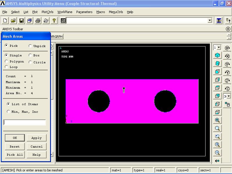
Next from Main Menu click Preprocessor - Meshing - Mesh - Areas - Free. Mesh Areas window appears. Pick the area and click OK.

As you can see the element sizes are not proper sizes. So the element sizes need to be reduced. Therefore to clear the current mesh, from Main Menu click Preprocessor - Meshing - Clear - Areas. Clear Areas window appears. Pick the area and click OK.

Next from Main Menu click Preprocessor - Meshing - Size Cntrls - ManualSize - Areas - All Areas. Element Sizes on All Selected Areas window appears. In Element edge length box enter 0.05m and click OK.

Next from Main Menu click Preprocessor - Meshing - Mesh - Areas - Free. Mesh Areas window appears. Pick the area and click OK.


8). From Main Menu click Preprocessor - Physics - Environment - Write. Physics write window appears. Enter Thermal for title and click OK.

From Main Menu click Preprocessor - Physics - Environment - Clear. Click OK. Physics Clear window appears. Click OK. Doing this clears all the information prescribed for the geometry, such as the element type, material properties, etc. It does not clear the geometry however, so it can be used in the next stage, which is defining the structural environment.

===========================================================
9). Now we need to convert the thermal element type to the corresponding element type for structural analysis. To do this, from Main Menu click Preprocessor - Element Type - Switch Elem Type. Switch Elem Type window appears. From Change element type list select Thermal to Struc option and click OK.

This will switch to the complimentary structural element automatically and create a structural element of LINK182 in Element Types window.

In Element Types window click on Options button. From Element Behavior list select Plane strs w/thk option and click OK and close Element Types window.

10). To define element properties, from Main Menu click Preprocessor - Real Constants - Add/Edit/Delete. Real Constants window appears. Click on Set 1 from list and click Edit.

PLANE182 is added to the list. Click OK.

Real Constant Set Number 1, for PLANE182 window appears. As the thickness of 0.01 is already entered. Click OK.

Close Real Constants window.

11). To define Structural Material Properties, from Main Menu click Preprocessor - Material Props - Material Models. Define Material Model Behavior window appears. From list select Structural - Linear - Elastic - Isotropic. Enter EX = 210e9 and PRXY = 0.3 and click OK.

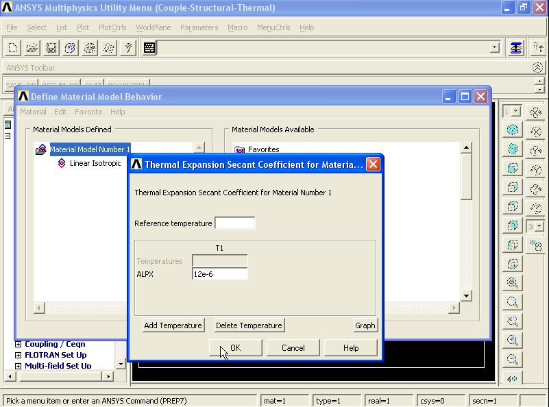
To define thermal expansion coefficient, from Define Material Model Behavior window, click Thermal Expansion - Secant Coefficient - Isotropic. Enter ALPX = 12e-6 and click OK.
Close Define Material Model Behavior window.

12). From Main Menu click Preprocessor - Physics - Environment - Write. Physics write window appears. Enter Structural in Physics file title and click OK.

13). From Main Menu Solution - Analysis Type - New Analysis. New Analysis window appears. From list select Static and click OK.

14). From Main Menu click Preprocessor - Physics - Environment - Read. Physics Read window appears. From list select THERMAL and click OK.

15). To apply Boundary Conditions, from Main Menu click Preprocessor - Loads - Define Loads - Apply - Thermal - Temperature - On Lines. Apply TEMP on Lines window appears. Pick the edges of the right circle and click OK.

Apply TEMP on Lines window appears. From list select TEMP and in Load TEMP value box enter -35C and click OK.

To apply Boundary Conditions to the left circle, from Main Menu click Preprocessor - Loads - Define Loads - Apply - Thermal - Temperature - On Lines. Apply TEMP on Lines window appears. Pick the edges of the left circle and click OK.

Apply TEMP on Lines window appears. From list select TEMP and in Load TEMP value box enter 150C and click OK.

===========================================================
Thermal Solution Stage:
16). From Main Menu click Solution - Solve - Current LS. Click OK to start solution. Close the window.

===========================================================
Post Processing Stage:
17). From Main Menu click General Postproc - Plot Results - Contour Plot - Nodal Solu. Contour Nodal Solution Data window appears. From list click DOF Solution - Nodal Temperature. Click OK.


Then from Main Menu click Finish.

18). From Main Menu click Preprocessor - Physics - Environment - Read. Physics Read window appears. From list select STRUCTURAL and click OK.

19). To apply Structural Boundary Conditions, from Main Menu click Preprocessor - Loads - Define Loads - Apply - Structural - Displacement - On Lines. Apply U, ROT on Lines window appears. Pick the edges of the right circle and click OK.

Apply U, ROT on Lines window appears. Select All DOF from list and click OK.

To apply Structural Boundary Conditions to the left circle, from Main Menu click Preprocessor - Loads - Define Loads - Apply - Structural - Displacement - On Lines. Apply U, ROT on Lines window appears. Pick the edges of the left circle and click OK.


From Main Menu click Preprocessor - Loads - Define Loads - Apply - Structural - Temperature - From Therm Analy. Apply TEMP from Thermal Analysis window appears. Click on Browse button.

Select the file which was created at the beginning of the analysis (Couple-Structural-Thermal.rth) and click Open.

Apply TEMP from Thermal Analysis window again appears. Click on OK to close the window.

Next from Main Menu click Preprocessor - Loads - Define Loads - Settings - Reference Temp. Reference Temperature window appears. Enter 25C in Reference Temperature box and click OK.

===========================================================
Structural Solution Stage:
From Main Menu click Solution - Solve - Current LS. Click OK to start solution. Close the window.

===========================================================
Post Processing Stage:
From Main Menu click General Postproc - Plot Results - Contour Plot - Nodal Solu. Contour Nodal Solution Data window appears. From list click DOF Solution - X-Component of displacement. Click OK.


Y-Component of displacement:

Displacement vector sum:

Stress - X-Component of stress:

Y-Component of stress:

XY Shear stress:

Von mises stress:

To animate the deformation, from Menu click PlotCtrls - Animate - Mode Shape...

Animate Mode Shape window appears. From left column select Stress and from right column select von mises and click OK.


==========================================================
The temperature distribution in a part can cause thermal stress effects (stresses caused by thermal expansion or contraction of the material). Examples of this phenomena include interference fit processes (also called shrink fits), where parts are mated by heating one part and keeping the other part cool for easy assembly. Another example is thermal creep, which is permanent deformation resulting from prolonged application of a stress below the elastic limit. An example of this is the behavior of metals exposed to mechanical loads and elevated temperatures over time.
Thermal stress effects can be simulated by coupling a heat transfer analysis (steady-state or transient) and a structural analysis (static stress with linear or nonlinear material models.
A steel link, with no internal stresses, is pinned between two solid structures at a reference temperature of 0 C (273 K). One of the solid structures is heated to a temperature of 75 C (348 K). As heat is transferred from the solid structure into the link, the link will attempt to expand. However, since it is pinned this cannot occur and as such, stress is created in the link. A steady-state solution of the resulting stress will be found to simplify the analysis.
Loads will not be applied to the link, only a temperature change of 75 degrees Celsius. The link is steel with a modulus of elasticity of 200 GPa, a thermal conductivity of 60.5 W/m*K and a thermal expansion coefficient of 12e-6 /K and the length of the link is 1m. The cross section of the link is square with 2cm side.

1). From Menu click File - Change Title... Change Title window appears. Enter Couple 1 for the title name and click OK.

The title name is appears at the bottom of the screen.

2). From Main Menu click Preferences. Preferences for GUI Filtering window appears. Select Thermal option and click OK.
2). To define Element Types, from Main Menu click Preprocessor - Element Type - Add/Edit/Delete. Element Types window appears. Click on Add button. Library of Element Types window appears. From left column select Link and from right column select 3D conduction 33 and click OK.

LINK33 is added to the Element Types window. Close this window.

3). To define element properties, from Main Menu click Preprocessor - Real Constants - Add/Edit/Delete. Real Constants window appears. Click on Add button.

Then select LINK33 and click OK.

Real Constant Set Number 1, for LINK33 window appears. In Cross-sectional area box enter 4e-4 and click OK.

Set 1 is added to the Real Constants window. Close the window.

4). To define Thermal properties of material, from Main Menu click Preprocessor - Material Props - Material Models. Define Material Model Behavior window appears. Click Thermal - Conductivity - Isotropic. Enter KXX = 60.5 and click OK. Then close Define Material Model Behavior window.

5). To create the Geometry, from Main Menu click Preprocessor - Modeling - Create - Keypoints - In Active CS. Create the following points: 1.(0,0,0) - 2.(1,0,0) and click OK.

Then connect these two points. From Main Menu click Preprocessor - Modeling - Create - Lines - Lines - Straight Lines. Create Straight Line window appears. Connect point 1 to point 2. Click OK.

6). To Mesh the model, from Main Menu click Preprocessor - Meshing - Mesh Tool. Mesh Tool window appears. Click on Lines Set button.

Element Size on Picked Lines window appears. Pick the line and click OK.

Element Size on Picked Lines window appears. In No. of element divisions box enter 10 and click OK.

From Mesh Tool window click on Mesh button.

Mesh Lines window appears. Pick the model and click OK.


===========================================================
7). From Main Menu click Preprocessor - Physics - Environment - Write. Physics Write window appears. In Physics file title box enter Thermal and click OK.

From Main Menu click Preprocessor - Physics - Environment - Clear. Physics Clear window appears. Click OK. Doing this clears all the information prescribed for the geometry, such as the element type, material properties, etc. It does not clear the geometry however, so it can be used in the next stage, which is defining the structural environment.

===========================================================
8). Now we need to convert the thermal element type to structural element type.
To do this, from Main Menu click Preprocessor - Element Type - Switch Elem Type. Switch Elem Type window appears. From Change element type list select Thermal to Struc option and click OK.

This will switch to the complimentary structural element automatically and create a structural element of LINK180 in Element Types window. Close the window.

9). To define Material Properties, from Main Menu click Preprocessor - Material Props - Material Models. Define Material Model Behavior window appears. From right column select Structural - Linear - Elastic - Isotropic. Enter EX = 200e9 and PRXY = 0.3 and click OK.

To define Thermal Expansion properties, in Define Material Model Behavior window click Thermal Expansion - Secant Coefficient - Isotropic. Enter ALPX = 12e-6 and click OK.

Close Define Material Model Behavior window.

10). From Main Menu click Preprocessor - Physics - Environment - Write. Physics Write window appears. In Physics file title box enter Structural and click OK.

===========================================================
11). To define analysis type, from Main Menu click Solution - Analysis Type - New Analysis. New Analysis window appears. Select Static and click OK.

Then from Main Menu click Preprocessor - Physics - Environment - Read. Physics Read window appears. Select Thermal from list and click OK.

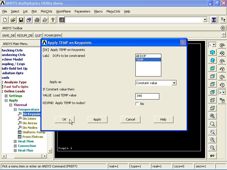
12). To apply thermal boundary conditions, from Main Menu click Preprocessor - Loads - Define Loads - Apply - Thermal - Temperature - On Keypoints. Apply TEMP on KPs window appears. Pick the left point and click OK.

Apply TEMP on Keypoints window appears. Select TEMP from list and in Load TEMP value box enter 348K and click OK.

===========================================================
Thermal Solution Stage:
13). Now the the problem will be solved thermally. From Main Menu click Solution - Solve - Current LS. Click OK to start solution. Close the window.

===========================================================
Post Processing Stage:
14). From Main Menu click Preprocessor - General Postproc - Plot Results - Contour Plot - Nodal Solu. Contour Nodal Solution Data window appears. Select DOF Solution - Nodal Temperature. Click OK.

The results is in Steady-State mode and that's why the temperature in all over the link is 348K.

In next stage from Main Menu click on Finish.

===========================================================
15). From Menu click File - Save as Jobname.db. This will cause the this analysis to be considered as current file. This information is saved in a file labelled Jobname.rth, were .rth is the thermal results file. Since the jobname wasn't changed at the beginning of the analysis, this data can be found as file.rth. We will use these results in determing the structural effects.

16). Then from Main Menu click Preprocessor - Physics - Environment - Read. Physics Read window appears. From list select Structural and click OK.

17). To apply boundary conditions, from Main Menu click Preprocessor - Loads - Define Loads - Apply - Structural - Displacement - On Keypoints. Apply U, ROT on KPs window appears. Pick the point number 1 and click OK.

Apply U, ROT on KPs window appears. Select All DOF option from list and click OK.

Again from Main Menu click Preprocessor - Loads - Define Loads - Apply - Structural - Displacement - On Keypoints. Apply U, ROT on KPs window appears. Pick the point number 2 and click OK.

Apply U, ROT on KPs window appears. Select UX option from list and click OK.

Next from Main Menu click Preprocessor - Loads - Define Loads - Apply - Structural - Temperature - From Therm Analy. Apply TEMP from Thermal Analysis window appears. Click on Browse button.

From window select file.rth and click Open.

Apply TEMP from Thermal Analysis window again appears. Click OK.

Next from Main Menu click Preprocessor - Loads - Define Loads - Settings - Reference Temp. Reference Temperature window appears. In Reference temperature box enter 273K and click OK.

===========================================================
Structural Solution Stage:
From Main Menu click Solution - Solve - Current LS. Click OK to start solution. Close the window.

===========================================================
Post Processing Stage:
From Main Menu click General Postproc - Element Table - Define Table. Element Table Data window appears. Click on Add button.

Define Additional Element Table Items window appears. From left column select By sequence num and from right column select LS, then enter 1 in front of LS, and click OK.

LS1 is added to the Element Table Data window. Close this window.

Next from Main Menu click General Postproc - Element Table - Plot Elem Table. Contour Plot of Element Table Data window appears. Click OK.

The maximum pressure is 180MPa and for all the link is constant.

Next from Main Menu click General Postproc - Element Table - List Elem Table. List Element Table Data window appears. From list select LS1 and click OK.

The table results appears.


Then select LINK33 and click OK.

Real Constant Set Number 1, for LINK33 window appears. In Cross-sectional area box enter 4e-4 and click OK.

Set 1 is added to the Real Constants window. Close the window.

4). To define Thermal properties of material, from Main Menu click Preprocessor - Material Props - Material Models. Define Material Model Behavior window appears. Click Thermal - Conductivity - Isotropic. Enter KXX = 60.5 and click OK. Then close Define Material Model Behavior window.

5). To create the Geometry, from Main Menu click Preprocessor - Modeling - Create - Keypoints - In Active CS. Create the following points: 1.(0,0,0) - 2.(1,0,0) and click OK.

Then connect these two points. From Main Menu click Preprocessor - Modeling - Create - Lines - Lines - Straight Lines. Create Straight Line window appears. Connect point 1 to point 2. Click OK.

6). To Mesh the model, from Main Menu click Preprocessor - Meshing - Mesh Tool. Mesh Tool window appears. Click on Lines Set button.

Element Size on Picked Lines window appears. Pick the line and click OK.

Element Size on Picked Lines window appears. In No. of element divisions box enter 10 and click OK.

From Mesh Tool window click on Mesh button.

Mesh Lines window appears. Pick the model and click OK.


===========================================================
7). From Main Menu click Preprocessor - Physics - Environment - Write. Physics Write window appears. In Physics file title box enter Thermal and click OK.

From Main Menu click Preprocessor - Physics - Environment - Clear. Physics Clear window appears. Click OK. Doing this clears all the information prescribed for the geometry, such as the element type, material properties, etc. It does not clear the geometry however, so it can be used in the next stage, which is defining the structural environment.

===========================================================
8). Now we need to convert the thermal element type to structural element type.
To do this, from Main Menu click Preprocessor - Element Type - Switch Elem Type. Switch Elem Type window appears. From Change element type list select Thermal to Struc option and click OK.

This will switch to the complimentary structural element automatically and create a structural element of LINK180 in Element Types window. Close the window.

9). To define Material Properties, from Main Menu click Preprocessor - Material Props - Material Models. Define Material Model Behavior window appears. From right column select Structural - Linear - Elastic - Isotropic. Enter EX = 200e9 and PRXY = 0.3 and click OK.

To define Thermal Expansion properties, in Define Material Model Behavior window click Thermal Expansion - Secant Coefficient - Isotropic. Enter ALPX = 12e-6 and click OK.

Close Define Material Model Behavior window.

10). From Main Menu click Preprocessor - Physics - Environment - Write. Physics Write window appears. In Physics file title box enter Structural and click OK.

===========================================================
11). To define analysis type, from Main Menu click Solution - Analysis Type - New Analysis. New Analysis window appears. Select Static and click OK.

Then from Main Menu click Preprocessor - Physics - Environment - Read. Physics Read window appears. Select Thermal from list and click OK.

12). To apply thermal boundary conditions, from Main Menu click Preprocessor - Loads - Define Loads - Apply - Thermal - Temperature - On Keypoints. Apply TEMP on KPs window appears. Pick the left point and click OK.

Apply TEMP on Keypoints window appears. Select TEMP from list and in Load TEMP value box enter 348K and click OK.
===========================================================
Thermal Solution Stage:
13). Now the the problem will be solved thermally. From Main Menu click Solution - Solve - Current LS. Click OK to start solution. Close the window.

===========================================================
Post Processing Stage:
14). From Main Menu click Preprocessor - General Postproc - Plot Results - Contour Plot - Nodal Solu. Contour Nodal Solution Data window appears. Select DOF Solution - Nodal Temperature. Click OK.

The results is in Steady-State mode and that's why the temperature in all over the link is 348K.

In next stage from Main Menu click on Finish.

===========================================================
15). From Menu click File - Save as Jobname.db. This will cause the this analysis to be considered as current file. This information is saved in a file labelled Jobname.rth, were .rth is the thermal results file. Since the jobname wasn't changed at the beginning of the analysis, this data can be found as file.rth. We will use these results in determing the structural effects.

16). Then from Main Menu click Preprocessor - Physics - Environment - Read. Physics Read window appears. From list select Structural and click OK.

17). To apply boundary conditions, from Main Menu click Preprocessor - Loads - Define Loads - Apply - Structural - Displacement - On Keypoints. Apply U, ROT on KPs window appears. Pick the point number 1 and click OK.

Apply U, ROT on KPs window appears. Select All DOF option from list and click OK.

Again from Main Menu click Preprocessor - Loads - Define Loads - Apply - Structural - Displacement - On Keypoints. Apply U, ROT on KPs window appears. Pick the point number 2 and click OK.

Apply U, ROT on KPs window appears. Select UX option from list and click OK.

Next from Main Menu click Preprocessor - Loads - Define Loads - Apply - Structural - Temperature - From Therm Analy. Apply TEMP from Thermal Analysis window appears. Click on Browse button.

From window select file.rth and click Open.

Apply TEMP from Thermal Analysis window again appears. Click OK.

Next from Main Menu click Preprocessor - Loads - Define Loads - Settings - Reference Temp. Reference Temperature window appears. In Reference temperature box enter 273K and click OK.

===========================================================
Structural Solution Stage:
From Main Menu click Solution - Solve - Current LS. Click OK to start solution. Close the window.

===========================================================
Post Processing Stage:
From Main Menu click General Postproc - Element Table - Define Table. Element Table Data window appears. Click on Add button.

Define Additional Element Table Items window appears. From left column select By sequence num and from right column select LS, then enter 1 in front of LS, and click OK.

LS1 is added to the Element Table Data window. Close this window.

Next from Main Menu click General Postproc - Element Table - Plot Elem Table. Contour Plot of Element Table Data window appears. Click OK.

The maximum pressure is 180MPa and for all the link is constant.

Next from Main Menu click General Postproc - Element Table - List Elem Table. List Element Table Data window appears. From list select LS1 and click OK.

The table results appears.

No comments:
Post a Comment